4. Diffusion
4. Diffusion. 4.1 Definition. Diffusion is defined as a process of mass transfer of individual molecules of a substance, brought about by random molecular motion and associated with a concentration gradient.

4. Diffusion
E N D
Presentation Transcript
4.1 Definition • Diffusion is defined as a process of mass transfer of individual molecules of a substance, brought about by random molecular motion and associated with a concentration gradient. • Spreading out, mixing. The diffusion of gases and liquids refers to their mixing without an external force.
4.2. Mechanisms • Diffusion could occur: • Throughout a single bulk phase (solution’s homogeneity). • Through a barrier, usually a polymeric membrane (drug release from film coated dosage forms, permeation and distribution of drug molecules in living tissues, passage of water vapor and gases through plastic container walls and caps, ultrafiltration).
4.2. Mechanisms • Diffusion through a barrier may occur through either: • Simple molecular permeation (molecular diffusion) through a homogenous nonporous membrane. This process depends on the dissolution of the permeating molecules in the barrier membrane. • Movement through pores and channels (heterogeneous porous membrane) which involves the passage of the permeating molecules through solvent filled pores in the membrane rather than through the polymeric matrix itself.
4.2. Mechanisms A B Diffusion through a homogenousnonporous membrane (A) and a porous membrane with solvent (usually water) filled pores (B)
4.2. Mechanisms • Both mechanisms usually exist in any system and contribute to the overall mass transfer or diffusion. • Pore size, molecular size and solubility of the permeating molecules in the membrane polymeric matrix determine the relative contribution of each of the two mechanisms.
4.2. Mechanisms • By combining the two mechanisms for diffusion through a membrane we can achieve a better representation of a membrane on the molecular scale. • A membrane can be visualized as a matted arrangement of polymer strands with branching and intersecting channels. An illustration of the microstructure of a cellulosemembrane used in the filtration processes showing the intertwining nature of fibers and aqueous channels
4.2. Mechanisms • Depending on the size and shape of the diffusing molecules, they may pass through the tortuous pores formed by the overlapping strands of the polymer. • The other alternative is to dissolve in the polymer matrix and pass through the film by simple diffusion. • Passage of steroidal molecules substituted with hydrophilic groups in topical preparation through human skin involves transport through the skin appendages (hair follicles, sebum ducts and sweat pores in the epidermis) as well as molecular diffusion through the stratum corneum.
4.3. Related Phenomena and Processes • Some processes and phenomena related to diffusion: • Dialysis: A separation process based on unequal rates of passage of solutes and solvent through microporous membranes (Hemodialysis). • Osmosis: Spontaneous diffusion of solvent from a solution of low solute concentration (or a pure solvent) into a more concentrated one through a membrane that is permeable only to solvent molecules (semipermeable).
4.3. Related Phenomena and Processes • Ultrafiltration: A separation process for colloidal particles and macromolecules where a hydraulic pressure is employed to force the solvent through a membrane that prevents the passage of large solute molecules (albumin and enzymes). • Microfiltration: A process similar to ultrafiltration employing slightly larger pore size membranes (100 nm to several micrometers). Used to remove bacteria from intravenous injections, food and drinking water
4.4. Fick’s First Law of Diffusion • Flux Jis the amount, M, of material flowing through a unit cross section, S, of a barrier in unit time, t. J = dM / S.dt • The units of the Flux J are g.cm-2.sec-1.
4.4. Fick’s First Law of Diffusion • According to the diffusion definition, the flow of material is proportional to the concentration gradient. • Concentration gradient represents a change of concentration with a change in location. • Concentration gradient is referred to as dc/dx where c is the concentration in g/cm3 and x is the distance in cm of movement perpendicular to the surface of the barrier ( i.e. across the barrier).
4.4. Fick’s First Law of Diffusion J dc/dx J = -D*(dc/dx)Fick’s First Law • In which D is the diffusion coefficient of the permeating molecule (diffusant, penetrant) in cm2/sec. • D is more correctly referred to as Diffusion Coefficient rather than constant since it does not ordinarily remain constant and may change with concentration. • The negative sign in the equation signifies that the diffusion occurs in the direction of decreased concentration. • Flux J is always a positive quantity (dc/dx is always negative). • Diffusion will stop when the concentration gradient no longer exists (i.e., when dc/dx = 0).
Diffusion and Molecular Properties • Diffusion depends on the resistance to passage of a diffusing molecule and is a function of the molecular structure of the diffusant as well as the barrier material. • Gas molecules diffuse rapidly through air and other gases. Diffusivities in liquids are smaller and in solids still smaller.
4.5. Fick’s Second Law of Diffusion • Fick’s first law examined the mass diffusion across a unit area of a barrier in a unit time (J). • Fick’s second law examines the rate of change of diffusant concentration with time at a point in the system (c/t) . • The diffusant concentration c in a particular volume element changes only as a result of a net flow of diffusing molecules into or out of the specific volume unit.
4.5. Fick’s Second Law of Diffusion C Input Output Volume element Bulk medium
4.5. Fick’s Second Law of Diffusion • A difference in concentration results from a difference in input and output. • The rate of change in the concentration of the diffusant with time in the volume element (c/t) equals the rate of change of the flux (amount diffusing) with distance (J/x) in the x direction. dc/dt = - dJ/dx
4.5. Fick’s Second Law of Diffusion dc/dt = - dJ/dx J = -D*(dc/dx) • Differentiating with respect to x dJ/dx = D*(d2c/dx2) • substituting dc/dt from the top equation dc/dt = D*(d2c/dx2)
4.5. Fick’s Second Law of Diffusion dc/dt = D*(d2c/dx2) • This equation represents diffusion in the x axis only. In order to describe diffusion in three dimensional space, Fick’s second law can be written as dc/dt = D*(d2c/dx2 +d2c/dy2 +d2c/dz2 )
4.5. Fick’s Second Law of Diffusion C Input Output Volume element Bulk medium
4.6. Steady state Diffusion • An important condition in diffusion is that of steady state • Fick’s first law gives the flux (or rate of diffusion throughout unit area) in the steady state of flow. • Fick’s second law refers in general to a change in concentration of diffusant with time, at any distance, x (i.e., a nonsteady state of flow). • Steady state may be described, however, in terms of the second law.
4.6. Steady state Diffusion • Diffusion Cells: • In a diffusion cell, two compartments are separated by a polymeric membrane. • The diffusant is dissolved in a proper solvent and placed in one compartment while the solvent alone is placed in the other. • The solution compartment is described as Donor Compartment because it is the source of the diffusant in the system while the solvent compartment is described as the Receptor Compartment.
4.6. Steady state Diffusion • In diffusion experiments, the solution in the receptor compartment is constantly removed and replaced with a fresh solvent to keep the concentration of the diffusant passing from the donor compartment at a low level. This is referred to as the Sink Condition.
4.6. Steady state Diffusion Donor Compartment Receptor Compartment Pure solvent Diffusant Solution Membrane Flux in Flux out Flow of solvent to maintain sink condition
4.6. Steady state Diffusion • As the diffusant passes through the membrane from the donor compartment (d) to the receptor compartment (r), the concentration in the donor compartment (Cd) will fall while the concentration in the receptor (Cr) will rise. • However, the concentration in the receptor compartment is always maintained at very low levels because of the sink condition. • This means that Cr << Cd
4.6. Steady state Diffusion • When the system has been in existence for a sufficient period of time (determined by the nature of barrier and the rate of removal of the diffusant by the sink system), the rate of change in concentration in the two compartments with time will become constant. • However, the concentration in the two compartments is not the same.
4.6. Steady state Diffusion dc/dt = D*(d2c/dx2) = 0 • Since D is not equal to (0), then d2c/dx2 should be 0. • Sinced2c/dx2 is a second derivative, and is equal to (0) the first derivative dc/dx should be a constant. • This means that the concentration gradient dc/dx across the membrane is constant (linear relationship between concentration c and distance or membrane thickness h)
4.6. Steady state Diffusion Receptor Compartment Donor Compartment C1 Cd High concentration of diffusant molecules C2 Cr h 0 Thickness of barrier
4.6. Steady state Diffusion • In such systems (diffusion cells), Fick’s first law may be written as: J = dM / S.dt = D *(C1-C2)/h • C1 and C2 are the concentrations within the membrane and are not easily measured. • However they can be calculated using the partition coefficient (K)and the concentrations on the donor (Cd) and receptor (Cr) sides which can be easily measured
4.6. Steady state Diffusion K = C1/Cd = C2/Cr • Replacing C1 and C2 with KCd and KCr dM / S.dt = D (C1-C2)/h = D(K Cd -K Cr)/h dM / S.dt = DK(Cd - Cr)/h dM / dt = DSK(Cd - Cr)/h
4.6. Steady state Diffusion • If the sink condition holds in the receptor compartment Cd>>Cr 0 and Cr drops out of the equation which becomes dM / dt = DSKCd /h • The term DK/h is referred to as the Permeability Coefficient or Permeability (P) and has the units of linear velocity (cm/sec). • The equation simplifies further to become dM / dt = PSCd
4.6. Steady state Diffusion • Permeability can be calculated from experimental data obtained from diffusion cells. - If Cdremains relatively constant throughout time, P can be obtained from the slope of a linear plot of M versus t. M = PS Cd t Cd = Cd(0) - (PSt/Vd) - If Cdchanges appreciably with time, then P can be obtained from the slope of log Cdversus t. log Cd = log Cd(0) - (PSt/2.303Vd)
Drug Release • The release of drug from a delivery system and subsequent bioabsorption involve factors of both dissolution and diffusion. • Diffusion is the main and most important mechanism involved in drug release from dosage forms. • Drug release occurs either from: (i) Film coated dosage forms (i.e. reservoir systems with zero order release mechanism) . (ii) Matrix type dosage forms represent a very important group of solid dosage forms where drug release is controlled by dissolution and diffusion.
Coated tablets Dissolution Polymeric membrane Diffusion Solid Core Saturated solution in equilibrium with solid core Unit Activity
Coated tablets • Drug release from these systems follows generally zero order kinetics which can be presented by the following equation: M = SDKCdt/h This behavior is presented in the straight dotted line presented in the following figure
Coated tablets Steady state with no lag time First order release Amount Diffused Steady state Nonsteady state Time Lag time tL
Coated tablets • However, these systems may not exhibit a zero order release in the initial stages (membrane hydration, dissolution of part of the solid core to create the saturated solution) and a lag time may be observed. • and the lag time is given by: tL = h2/6D When diffusivity can be calculated, presuming a knowledge of the membrane thickness, h • Also, knowing P, the thickness h can be calculated from tL = h/6P
Coated tablets • Drug release from these systems follows generally zero order kinetics which can be presented by the following equation: M = SDKCd(t-tL)/h This behavior is presented in the straight solid line presented in the previous figure • If the excess solid in the dosage form is depleted, the activity () decreases as the drug diffuses out of the system and the release rate falls exponentially (First order release).
Matrix type dosage forms Figure – Drug eluted from a homogeneous polymer matrix
Matrix type dosage forms • A matrix type dosage form is a drug delivery system in which the drug is homogenously dispersed throughout a polymeric matrix. • The drug in the polymeric matrix is assumed to be present at a total concentration A (mg/cm3). Part of the drug is soluble in the polymeric matrix and the concentration of the dissolved drug in the polymeric matrix is Cs (mg/cm3). Csis the solubility or saturation concentration of the drug in the matrix.
Matrix type dosage forms • To be released from the delivery system, the drug molecules have to dissolve and diffuse out from the surface of the device. • As the drug is released, the boundary that forms between the drug and empty matrix recedes into the tablet and the distance for diffusion becomes increasingly greater. Therefore, drug release will be faster in the initial stages and become slower later as the remaining drug molecules should cross longer distances than the first drug molecules. The release in these systems is best described by Higuchi.
Matrix type dosage forms Schematic presentation of the solid matrix and its receding boundary as the drug diffuses from the dosage form
Matrix type dosage forms • Higuchi (1960,1961) developed an equation to describe drug release from such matrix systems based on Fick’s 1st Law: dM/S.dt = dQ/dt = DCs/h where dQ/dt is the rate of drug released per unit area of exposed surface of the matrix.
Matrix type dosage forms • The amount of drug released (dQ) as the drug boundary recedes by a distance of (dh) is given by the approximate linear expression: dQ = A.dh – ½(Cs.dh) = dh.(A –½Cs) • The final form of the equation is known as the Higuchi equation. It is represented as follows: Q = [D(2A – Cs) Cst] ½
Matrix type dosage forms • And the instantaneous rate of release of a drug at time t is obtained by differentiating the above equation to give: dQ/dt = ½[D(2A-Cs)Cs/t]½ • The rate of release, dQ/dt, can be altered by increasing or decreasing the drug solubility Cs in the polymer by complexation. • The total amount A of drug is also seen to affect the rate of release.
Matrix type dosage forms • Usually A >> Cs and so both amount and rate equation reduces to: Q = (2DACst)½ dQ/dt = (ADCs/2t)½ • The equations indicate that the amount of drug released is proportional to the square root of: • The total amount of drug in unit volume of matrix (A) • The diffusion coefficient of the drug in the matrix (D) • The solubility of drug in the polymer matrix (Cs)
Matrix type dosage forms Example 13-6; Martin’s 6th ed.: • What is the amount of drug per unit area, Q, released from a tablet matrix at time t = 120 min? The total concentration of drug in the homogeneous matrix, A, is 0.02 g/ cm3. The drug’s solubility, Cs, is 1.0 x 10⁻³ g/ cm3 in the polymer. The diffusion coefficient, D, of the drug in the polymer matrix at 25°C is 6.0 x 10⁻⁶ cm2/sec or 360 x 10-6 cm2/min. Q = (2DACst)½ Q = (2* 360x10-6* 0.02* 1 x 10-3* 120)1/2 Q = 1.3 x 10⁻³ g/cm2 (b) What is the instantaneous rate of drug release occurring at 120 min? dQ/dt = (ADCs/2t)½ dQ/dt = (360x10-6* 0.02* 1 x 10-3/ 2*120)1/2 dQ/dt = 5.5 x 10⁻⁶ g cm-2 min-1
Matrix type dosage forms • The above discussion applies to drug diffusion in homogenous matrices; that either gradually (very slowly) erodes or even not erodes at all; and leaches the drug to the bathing medium through “ straight through” linear pores. • For granular matrices where drug diffuses through interstitial channels or pores, the diffusion distance is increased due to branching and bending of pores. In such systems, by the drug is leached and depleted, a shell of polymer with empty pores is left. • The volume and length of the matrix channels can be accounted for by adding new terms to the Higuchi equation.