Download
1 / 49
500 likes | 689 Vues
Toward 0-norm Reconstruction, and A Nullspace Technique for Compressive Sampling. Christine Law Gary Glover Dept. of EE, Dept. of Radiology Stanford University. Outline. 0-norm Magnetic Resonance Imaging (MRI) reconstruction. Homotopic Convex iteration Signal separation example

E N D
Toward 0-norm Reconstruction, and A Nullspace Technique for Compressive Sampling Christine Law Gary Glover Dept. of EE, Dept. of Radiology Stanford University
Outline • 0-norm Magnetic Resonance Imaging (MRI) reconstruction. • Homotopic • Convex iteration • Signal separation example • 1-norm deconvolution in fMRI. • Improvement in cardinality constraint problem with nullspace technique.
k = 2 n Shannon vs. Sparse Sampling • Nyquist/Shannon : sampling rate ≥ 2*max freq • Sparse Sampling Theorem: (Candes/Donoho 2004) Suppose x in Rn is k-sparse and we are given m Fourier coefficients with frequencies selected uniformly at random. If m ≥ k log2 (1 + n / k) then reconstructs x exactly with overwhelming probability.
1 week Rat dies 1 week after drinking poisoned wine Example by Anna Gilbert
x1 x2 x3 x4 x5 x6 x7 y1 y2 y3
k=1 n=7 m=3 x1 x2 x3 x4 x5 x6 x7 y1 y2 y3
Reconstruction by Optimization • Compressed Sensing theory (2004 Donoho, Candes): under certain conditions, y are measurements (rats) x are sensors (wine) Candes et al. IEEE Trans. Information Theory 2006 52(2):489 Donoho. IEEE Trans. Information Theory 2006 52(4):1289
For p-norm, where 0 < p < 1 Chartrand (2006) demonstrated fewer samples y required than 1-norm formulation. Chartrand. IEEE Signal Processing Letters. 2007: 14(10) 707-710. 0-norm reconstruction • Try to solve 0-norm directly.
method method method Homotopic Homotopic Homotopic Trzasko (2007): Rewrite the problem where r is tanh, laplace, log, etc. such that Trzasko et al. IEEE SP 14th workshop on statistical signal processing. 2007. 176-180.
Homotopic function in 1D Start as 1-norm problem, then reduce s slowly and approach 0-norm function.
when is big (1st iteration), solving 1-norm problem. reduce to approach 0-norm solution. Demonstration x∆ original
Example 1 subsampled original
1-norm recon 1-norm result: use 4% Fourier data error: -11.4 dB 542 seconds Homotopic result: use 4% Fourier data error: -66.2 dB 85 seconds homotopic recon Fourier sample mask Zero-filled Reconstruction
Example 2 • Angiography • 360x360, 27.5% radial samples original
reconstruction homotopic method: error: -26.5 dB, 101 seconds original 27.5% samples 360x360 reconstruction 1-norm method: error: -24.7 dB, 1151 seconds
Convex Iteration Chretien, An Alternating l1 approach to the compressed sensing problem, arXiv.org . Dattorro, Convex Optimization & Euclidean Distance Geometry, Meboo.
Convex Iteration demo use 4% Fourier data error: -104 dB 96 seconds Fourier sample mask reconstruction zero-filled reconstruction
as convex iteration 1-norm formulation
= + u Signal Construction Cardinality(steps) = 7 Cardinality(cosine) = 4 u∆ uD
Minimum Sampling Rate m/k m measurements k cardinality n record length k/n Donoho, Tanner, 2005. Baron, Wakin et al., 2005
Signal Separation by Convex Iteration Cardinality(steps) = 7 Cardinality(cosine) = 4 m=28 measurements m/n= 0.1 subsample m/k= 2.5 sample rate k/n = 0.04sparsity
u∆ uD 1-norm -241dB reconstruction error Convex iteration TV only DCT only
functional Magnetic Resonance Imaging (fMRI) Haemodynamic Response Function (HRF)
How to conduct fMRI? Stimulus Timing Huettel, Song, Gregory. Functional Magnetic Resonance Imaging. Sinauer.
How to conduct fMRI? Stimulus Timing
Neural activity Signalling Vascular response BOLD signal Vascular tone (reactivity) Autoregulation Blood flow, oxygenation and volume Synaptic signalling arteriole B0 field glia Metabolic signalling End bouton dendrite venule What does fMRI measure?
rest task Oxygenated Hb Deoxygenated Hb fMRI signal origin Oxygenated Hb Deoxygenated Hb
Haemodynamic Response Function (HRF) Canonical HRF Stimulus Timing Predicted Data = = Time
Time Actual measurement Prediction Signal Intensity Time Time Which part of the brain is activated? http://www.fmrib.ox.ac.uk/
Variability of HRF Stimulus Timing Measurement Actual HRF = HRF calibration
Discrete wavelet transform Wh 1 0 (d) 10 0 -10 W: Coiflet E: monotone cone Dh y Deconvolve HRF h D(: , 1) D: convolution matrix
W: Coiflet wavelet E: monotone cone D: convolution matrix Dh Deconvolve HRF h smoothness D(:,1) 1 0 stimulus timing y 10 0 -10 measurement
HRF deconvolution … HRF deconvolution … … in vivo deconvolution results HRF calibration Time (s) Time (s)
Cardinality Constraint Problem 1 5 1 3 b A 3 x 5 A = b = A(:,2) * rand(1) + A(:,5) * rand(1)
= Find x with desired cardinality e.g. k = 2, want
From the Range perspective … In general, 1 1 n=5 3 b A x m=3 5 Check every pair for k = 2 Possible # solution:
5 A 3 Particular soln. General soln. Nullspace Perspective 2 = 0 Z 5
Z = 0.57 0.34 -0.03 -0.26 -0.16 0.02 -0.68 -0.63 0.22 0.47 xp = 0.34 1.11 -0.30 0 0
How to find intersection of lines? Sum of normalized wedges
Znew = Z * randn(2); Znew = -0.41-0.18 -0.80-0.30 0.48 0.19 -0.26-0.07 1.00 0.37 Z = -0.59 -0.36 0.06 -0.55 0.15 0.36 0.74 -0.08 -0.27 0.66 x = 0.34 1.11 -0.30 0 0 x = 0 0.68 0 0 0.51
Summary • Ways to find 0-norm solutions other than 1-norm (homotopic, convex iteration) • fewer measurements • faster • In cardinality constraint problem, convex iteration and nullspace technique success more often than 1-norm.