Download
1 / 54
570 likes | 758 Vues
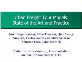
Urban Freight Tour Models: State of the Art and Practice. José Holguín-Veras, Ellen Thorson, Qian Wang, Ning Xu, Carlos González-Calderón, Iván Sánchez-Díaz, John Mitchell Center for Infrastructure, Transportation, and the Environment (CITE). Outline. 2. Introduction, Basic Concepts

E N D
Urban Freight Tour Models: State of the Art and Practice José Holguín-Veras, Ellen Thorson, Qian Wang, Ning Xu, Carlos González-Calderón, Iván Sánchez-Díaz, John Mitchell Center for Infrastructure, Transportation, and the Environment (CITE)
Outline 2 • Introduction, Basic Concepts • Urban Freight Tours: Empirical Evidence • Urban Freight Tour Models • Simulation Based Models • Hybrid Models • Analytical Models • Analytical Tour Models • Conclusions
R3 R2 Basic Concepts R1 S-2 R4 R5 S-1 Notation: S-3 Loaded vehicle-trip • A supplier sending shipments from its home base (HB) to six receivers • The goal is to capture both the underlying economics of production and consumption, and realistic delivery tours Empty vehicle-trip R6 Commodity flow Consumer (receiver) HB
Characterization of Urban Freight Tours (UFT) • Number of stops per tour depends on: Country, city, type of truck, the number of trip chains, type of carrier, service time, and commodity transported New York City Amsterdam Denver Alphen Apeldoorn Schiedam
Characterization of Urban Freight Tours (UFT) • Denver, Colorado (Holguín-Veras and Patil,2005): • Port Authority of NY and NJ (HV et al., 2006): • By type of company: • Common carriers: 15.7 stops/tour • Private carriers: 7.1 stops/tour • By origin of tour: • New Jersey: 13.7 stops/tour • New York: 6.0 stops/tour
Characterization of Urban Freight Tours (UFT) • NYC and NJ (Holguin-Veras et al. 2012): • Average: 8.0 stops/tour 12.6%: 1 stop/tour • 54.9%: < 6 stops/tour 8.7% do > 20 stops • Parcel deliveries: 50-100 stops/tour
Urban Freight Tour Models • The UFT models could be subdivided into: • Simulation models • Hybrid models • Analytical models
Simulation Models • Simulation models attempt to create the needed isomorphic relation between model and reality by imitating observed behaviors in a computer program • Examples include: • Tavasszy et al. (1998) (SMILE) • Boerkamps and van Binsbergen (1999) (GoodTrip) • Ambrosini et al., (2004) (FRETURB) • Liedtke (2006) and Liedtke (2009) (INTERLOG)
Hybrid Models • Hybrid models incorporate features of both simulation and analytical models (e.g., using a gravity model to estimate commodity flows, and a simulation model to estimate the UFTs) • Examples include: • van Duin et al. (2007) • Wisetjindawat et al. (2007) • Donnelly (2007)
Analytical Models • Analytical models attend to achieve isomorphism using formal mathematic representations based on behavioral, economic, or statistical axioms • Two main branches: • Spatial Price equilibrium models (disaggregate) • Entropy Maximization models (aggregate) • Examples include: • Holguín-Veras (2000), Thorson (2005) • Xu (2008), Xu and Holguín-Veras (2008) • Holguín-Veras et al. (2012) • Wang and Holguín-Veras (2009), Sanchez and Holguín-Veras (2012)
Entropy Maximization Tour Flow Models • Based on entropy maximization theory (Wilson, 1969; Wilson, 1970; Wilson, 1970) • Computes most likely solution given constraints • Key concepts: • Tour sequence: An ordered listing of nodes visited • Tour flow: The flow of vehicle-trips that follow a sequence • The problem is decomposed in two processes: • A tour choice generation process • A tour flow model
Entropy Maximization Tour Flow Model • Tour choice: To estimate sensible node sequences • Tour flow: To estimate the number of trips traveling along a particular node sequence Tour choice generation Tour flows
Entropy Maximization Tour Flow Model 20 • Definition of states in the system:
Entropy Maximization Tour Flow Model • The equivalent model of formulation 2: 22 MIN Subject to: Trip production constraints Total travel time constraint Total handling time constraint
Entropy Maximization Tour Flow Model • First-order conditions (tour distribution models) • Traditional gravity trip distribution model 23 Formulation 1: Formulation 2: Formulation 1 and the traditional GM model have exactly the same number of parameters
Entropy Maximization Tour Flow Model 24 • The optimal tour flows are found under the objective of maximizing the entropy for the system • The tour flows are a function of tour impedance and Lagrange multipliers associated with the trip productions and attractions along that tour • Successfully tested with Denver, Colorado, data: • The MAPE of the estimated tour flows is less than 6.7% given the observed tours are used • Much better than the traditional GM
Case Study: Denver Metropolitan Area 25 • Test network • 919 TAZs among which 182 TAZs contain home bases of commercial vehicles • 613 tours, representing a total of 65,385 tour flows / day • Calibration done with 17,000 tours (from heuristics) • Estimation procedure • Sorting input data: aggregate the observed tour flows to obtain trip productions and total impedance • Estimation: estimate the tour flows distributed on these tours using the entropy maximization formulations • Assessing performance: compare the estimated tour flows with the observed tour flows
Performance of the Models • Estimated vs. observed tour flows
TD-FTS Model • Bi-objective Program: Possible combinations of flow Function to replicate TD traffic counts Trip Production Constraint I can drop Trip Attraction Constraint Impedance Constraint
TD-FTS Model • Multi-attribute Value formulation: Utility function from DM Trip Production Constraint per Industry Impedance Constraint
Application to the Denver Region • TD-FTS MAPE’s: 0.8%-76.1% • Static Entropy Maximization (S-EM): MAPE’s 31.2%-117% • Gravity Model (DCGM): MAPE 79.5% • Temporal aspect better captured using TD-FTS
Multiclass traffic • Multiclass: two or more classes of travelers with different behavioral or choice characteristics • Vehicle classes are related under the same objective function • Multiclass equilibrium demand synthesis (MEDS) 33
Link Travel Cost • Travel time function depends on the vector of traffic flows for passenger cars and trucks • The travel cost is affected by the value of time of each one of the classes • The formula is a second order Taylor expansion of a general link-performance function Where: Xt: Vector of truck traffic flow Xc: Vector of passenger cars traffic flow 34
Multiclass Equilibrium • In a multiclass equilibrium, the cost functions of the modes are asymmetric, traffic flows interact • The user optimal assignment cannot be written as an optimization problem • The User Equilibrium (UE) problem could be addressed using a Variational Inequality (VI) Problem 35
Link Travel Cost • Although the vehicles share the transportation network and the travel time is the same (in equilibrium), the travel cost will be affected by the value of time of each one of the partiesvalue of time • Considering paths, the cost functions for truck tours and passenger cars will be given by: In a multiclass equilibrium, the cost functions of modes are asymmetric, traffic flows interact. UE Variational Inequality Where: :A binary variable indicating whether tour m uses link a :A binary variable indicating whether trip from i to j uses link a 36
Multiclass EM Formulations • The multiclass EM formulations is given by: Where: W: System entropy that represents the number of ways of distributing commercial vehicles tour flows and passenger cars flows Tt: Total number of commercial vehicle tour flows in the network; Tc: Total number of passenger cars flows in the network; tm : Number of commercial vehicle journeys (tour flows) following tour m; Tij : Number of car trips between i and j
Multiclass Equilibrium ODS Formulations The objective is to find the most likely ways to distribute tours considering congestion Min Subject to Subject to VI problem to obtain a UE condition for cars and trucks
General principles • The models estimate commodity flows and vehicle trips that arise under competitive market equilibrium • Conceptual advantages: • Account for tours • Provide a coherent framework to jointly model the joint formation of commodity flows and vehicle trips • Based on the seminal work of Samuelson (1952), as it seeks to maximize the economic welfare associated with the consumption and transportation of the cargo, taking into account the formation of UFTs
Two flavors • Independent Shipper-Carrier Operations: • Carrier and Shipper are independent companies • Carrier travels empty from its base to pick up cargo at shipper’s location(s) • Carrier delivers cargo to shipper’s customers • Carrier travels empty back to its base • Integrated Shipper-Carrier Operations: • Carrier and Shipper are part of the same company • Carrier is loaded at shipper’s location(s) • Carrier delivers cargo to shipper’s customers • Carrier travels empty back to its base
Legend: Integrated Shipper-Carrier Operations Supplier Receiver Empty trips • Five suppliers deploy tours from their bases (rhomboids) to distribute the cargo they produce to various consumer (demand) nodes (circles) Loaded trips made by suppliers (Contested nodes are shown as shaded circles)
Notation: p2 p3 A Spatial Price Equilibrium UFT Model Loaded Vehicle-trip eip2 eip3 Empty Vehicle-trip p4 eip4 • Samuelson’s model is reformulated to consider freight tours. A supplier i sends a cargo (eip1, eip2, eip3, and eip4) to different customers (p1, p2, p3, and p4) Commodity flow p1 eip1 i Supplier The cost of delivering to p3 is not the (path) cost along i-p1-p2-p3. It it is the (incremental) cost from p2 to p3, plus part of the empty trip cost.
A Spatial Price Equilibrium UFT Model (P1) MAX (Social Welfare) Subject to: (Area under excess supply function) (Excess supply) (Delivery cost to demand node) (Linking flows to vehicle-trips) (Tour length constraint) This term is equal to the summation of tour costs. Thus, it could be replaced by the summation of tour costs, which allows to eliminate the delivery cost constraint (Capacity constraint) (Conservation of flow) (Integrality) (Non-negativity)
A Spatial Price Equilibrium UFT Model (P2) MAX Subject to: (Net Social Payoff) (Area under excess supply function) (Excess supply) (Linking flows to vehicle-trips) (Tour length constraint) (Capacity constraint) (Conservation of flow) (Integrality) (Non-negativity)
However… • P2 is a nasty combinatorial and non-linear problem that is notoriously difficult to solve • To solve it, frame it as: • A dispersed SPE problem • A problem of profit maximization subject to competition (which is equivalent to the NSP formulation produced by Samuelson) • A dynamic problem in which competitors adjust decisions based on the market competition results • Use heuristics
Heuristic Solution Approach (Dispersed SPE) First-stage: Production level, prices, profit margins, net profits Initialization: Assume prices Phase 1: Initialization of TS, Generate initial solutions Profit-maximizing routing: Phase 2: Initial Improvement: Perform neighborhood search procedure Phase 3: Second Improvement, 2-Opt procedure and repeat 2 Phase 4: Intensification, Perform neighbor search on solutions from 3 No Convergence? Yes Market competition: Compute purchases from suppliers No Production dynamics: Update production level Equilibrium? Second-stage pricing: Compute optimal prices, profit margins No Yes Production dynamics: Update production level Equilibrium? STOP
Equilibrium Results Two suppliers, four customers Vehicle-tours (1.61, .47) (2.84, .89) (2.39, .10) (6.41, .10) (5.16, .10) (2.24, .73) (3.59, .97) C4 (3.76, .10) C4 Commodity flows and prices
Conclusions 50 • There are reasons to be optimistic: • The community is cognizant of the need to model tours • Collecting data and developing tour models • However: • The models developed are still in need of improvements • The data collected are small and not comprehensive • Simulations and hybrid models require better behavioral foundations that are not always validated • The most theoretically appealing models present significant computational challenges to be overcome • Entropy Maximization models offer an interesting avenue, though disregarding commodity flows