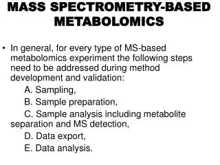
Basic principles of NMR-based metabolomics

1. NTDR, 2012 Basic principles of NMR-based metabolomics Nils Nyberg NPR, Department of Drug Design and Pharmacology

2. NTDR, 2012 Outline • NMR as universal detector • Top-down approach in science • Metabolomics and metabonomics • Case story: starved ewes and fat lambs • Step-by-step procedure in data handling • Processing • Export/import • Calibration • Baseline adjustment • Projection of data to a common axis • Integration and merging of buckets • PCA

3. NTDR, 2012 Basic principles of NMR-based metabolomics • Metabolome • The complete set of small-molecule metabolites in a biological system • Metabolomics, proteomics, transcriptomics, … • Metabolic profile, metabolic fingerprint • A quantitative determination of the metabolome in a sample or an individual • Metabonomics • Quantitative measurement of metabolic response to stimuli or genetic modification… • Toxicology • Disease diagnostics • Functional genomics (determination of phenotypes) • Nutrigenomics (human diet, drugs and microflora) • Metabonomics ~ metabolomics ~ metabolic profiles

4. NTDR, 2012 The universal detector • NMR: the most universal detector for small metabolites • No physical separation of analytes! • Robust => reproducible results • Directly quantitative • Simple sample preparation • Information rich • Not as sensitive as mass spectrometry • Expensive • NMR is good for a top-down approach • Study the whole system first, before breaking it into smaller pieces

5. NTDR, 2012 Starved ewes and fat lambs • Undernutrition during fetal development is associated with increased risk of metabolic diseases later in life. • Dutch winter famine 1944 • Obesity at the age of 50 y in men and women exposed to famine prenatally, Am J Clin Nutr 1999;70:811–16. • Coronary heart disease, hypertension, and type 2 diabetes. • Consequences of “programming,” whereby a stimulus or insult at a critical, sensitive period of early life has permanent effects on structure, physiology, and metabolism. • Metabolic programming • Phenotypic alterations by fetal adaption • Higher risk of obesity and diabetes if mismatched diet (programmed to cope with famine, exposed to hypernutrition)

6. NTDR, 2012 Starved ewes and fat lambs • Hypothesis: • Metabolic programming by feed restriction leads to changed metabolic pathways • The changes can be studied by acquiring NMR spectra of urine • Sheep as animal model system • Before birth:Ewes well fed or starved (50% of energy) • After birth: Normal diet or “High fat, high carbohydrate” diet

7. NTDR, 2012 Starved ewes and fat lambs: results • 164 NMR spectra • Repeats at 2 and 6 months

8. NTDR, 2012 Starved ewes and fat lambs: results • Principal Component Analysis (PCA) • Data reduction, keep the variance • Display the relationships between samples

9. NTDR, 2012 Starved ewes and fat lambs: results • Age: 2 months, adopting to ruminant digestion • Separation depending on diet,   /  • Some samples ahead,  separated from 

10. NTDR, 2012 Data handling: procedures and terms • From FID’s to one table

11. NTDR, 2012 Data handling: procedures and terms • Keep track of your samples and data! • Enter title or label for each sample • FID’s to spectra: • Window function, Fourier transform, phasing, base line adjustment • Make spectra comparable • Calibration of ppm-scale • Project data on a common axis • Normalize • Compress data/simplify spectra • Integrate (binning, buckets) • Simplify calculations/interpretation of models • Mean center • Scaling

12. NTDR, 2012 FID’s to spectra • Use the same processing parameters for all spectra! • Window function with parameters • Exponential Multiplication with a line broadening factor of 1 Hz • Number of data points in the final spectrum • 32768 data points/20 ppm/600 MHz = 2.7 data points/Hz • Make sure the peaks are properly defined.

13. NTDR, 2012 FID’s to spectra • Adjust each spectrum individually • Phasing: Adjust only zeroth-order phase constant if possible

14. NTDR, 2012 FID’s to spectra • Base line adjustment • Make sure the base line is represented in the spectrum (large SW) • Use a simple function (2nd or 3rd order polynomial)

15. NTDR, 2012 Calibration of ppm-scale • Select a reference peak • In all spectra • TMS, DSS or Residual solvent signal • Sharp, well resolved • Global shift (error in lock position) • Local shift (day to day variation in lock)

16. NTDR, 2012 Project data on a common axis • Discrete data points in different spectra are not necessarily aligned • Normally a very small effect

17. NTDR, 2012 Project data on a common axis

18. NTDR, 2012 Project data on a common axis

19. NTDR, 2012 Project data on a common axis

20. NTDR, 2012 Normalization • Make data directly comparable with each other • by removing known variation • by reducing unknown variation • row-wise operation (for each sample) • Variation caused by • different amounts/concentrations/volumes • instrument settings (tuning/matching, gain) • Variation expressed as • additive effects (base line) • multiplicative effects • Context dependent processing! • urine, serum, juice, … • depending on the type of samples, sampling schemes and sample preprocessing

21. NTDR, 2012 Some Normalization schemes • Normalize to • constant sum • constant squared sum • highest signal • Find a common constant feature in the spectra • internal standard • invariant metabolite • e.g. urinary creatinine/body weight

22. NTDR, 2012 Normalization • Be pragmatic – if it works, it’s probably ok! • But make sure the sampling and analysis parameters are kept constant • Some normalization schemes will introduce new correlations • Normalize to constant sum = if one signal increases, others are decreased

23. NTDR, 2012 Binning • Binning = Bucketing = Integration of spectral ranges • Reduce data set • typical spectra: 65536 data points (64k) • binned data ~200 data points • Remove variability of chemical shifts • temperature • pH • concentration • overall composition of samples (salt, proteins,…) • Reduce effects of differences in shimming • the area of a peak is a more robust measure than intensity value of each point

24. NTDR, 2012 Binning • Integration into smaller ranges • Bucketing or binning • Start with equidistant ranges, ~0.01-0.05 ppm • Combine vicinal buckets with a high degree of co-variation

25. NTDR, 2012 Mean/median centering • Removes (subtracts) the mean/median value of each variable • Operates on the columns of the data matrix (for each variable/bucket) • Centering of the data gives more stable numerical solutions for the PCA (and other transformations). • If not used – the first pc will be the mean spectrum… • Use median centering for a more robust centering • less sensitive to outliers

26. NTDR, 2012 Centering • Raw data, before centering

27. NTDR, 2012 Centering • Mean centered

28. NTDR, 2012 Centering • Median centered

29. NTDR, 2012 Scaling • Scaling sets the weighting (importance) of each variable in the models • For NMR-spectroscopic data • the largest signals have the highest variance • small signals have low variance • noise have lowest variance

30. NTDR, 2012 Auto scaling • Auto scaling (variables divided by standard deviation, variance set to 1).

31. NTDR, 2012 Pareto scaling • Pareto scaling (variables divided by the square root of the standard deviation).

32. NTDR, 2012 Log transform • The data range is ’compressed’ by calculation of the logarithmic values before centering.

33. NTDR, 2012 Scaling • Centering • Removes the offset in the data • Highlights the differences within each variable • Auto scaling • Sets the variance of each variable to unity. • Inflates the noise. • All signals equally important. • Pareto scaling • Reduce relative importance of large values. • Scaling effect between no scaling (only centering) and auto scaling.

34. NTDR, 2012 PCA • Principal Component Analysis (PCA) • Calculate scores and loadings • Data reduction (from 65000 data points to two…) • Keep the variance, don’t show the noise • Display the relationships between samples Loadings S X (systematic + random variation)

35. NTDR, 2012 PCA • Principal Component Analysis (PCA) • Calculate scores and loadings • Data reduction (from 65000 data points to two…) • Keep the variance, don’t show the noise • Display the relationships between samples Loadings S X (systematic variation) E (random variation)

36. NTDR, 2012 PCA • Principal Component Analysis (PCA) • Calculate scores and loadings • Data reduction (from 65000 data points to two…) • Keep the variance, don’t show the noise • Display the relationships between samples