Download
1 / 22
741 likes | 1.45k Vues
Training course in fish stock assessment and fisheries management. National Institute of Oceanography and Fisheries Fish population Dynamics Lab 10-14 November, 2013 ns. Su rplus Production models (Biomass Dynamic Models ). Prof. Dr. Sahar Fahmy Mehanna Head of fish population dynamics lab

E N D
Training course in fish stock assessment and fisheries management National Institute of Oceanography and Fisheries Fish population Dynamics Lab 10-14 November, 2013ns
Surplus Production models(Biomass Dynamic Models) Prof. Dr. SaharFahmyMehanna Head of fish population dynamics lab National Institute of Oceanography and Fisheries
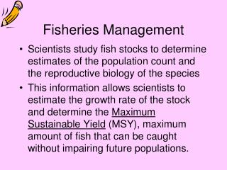
Surplus Production models • The level of the biomass of a population at time t+1 will depend to different phenomena. • While recruitment and individual growth contribute to its increase • mortality due to both natural causes and removals by fishing activity will contribute to its decline
Surplus Production models Bt+1 = Bt + Recruitment + Growth effects - Natural Mortality – Catch When there is no fishing, the combination of recruitment and growth is calledProduction Bt+1 = Bt + Production (P) - Natural Mortality (M)
Surplus Production models In the case P>M, the population will grow. The “Surplus Production” is defined as the increased amount of the population biomassin the absence of fishing or the amount of catch that can be harvested keeping biomass constant. Bt+1 = Bt+ Surplus Production – Catch in the case Catch > SurplusProduction, the biomass willdecrease.
Surplus Production models • Data requirements • In general use data on catch and effort • Equilibrium • Problems with quantification of effective effort • Multispecies-multigear fisheries (target, spatial and temporal changes…)
Some definitions Catch= landed fraction + discards + undefined incidental deaths Effort: Fishing effort (f) is the labour, vessels, skill and technology used in catching fish. One unit of fishing effort removes a certain constant fraction of a stock this effort is directly related to the fishing mortality (F) through a constant called catchability coefficient (q) Is catchability constant along time?
Some definitions F = qf q is the fraction of F produced by a unit of effort hence q may be a different value depending on which unit of effort is used! The choice of a suitable unit of effort
Catch Annual catches (avoidance of errors) due to: • Under-reporting (critical for management with TAC’s) • Discard at sea (individuals under legal size) • Not quantified incidental deaths (fish that is able to escape but successively will die due to bad conditions)
Effort • Definition of effort for such gear (trawlers, gill nets, hooks, traps) • Partitioning among species and fisheries • Standardization by vessels characteristics • Technological improvements along time
The more classical relationship between stock biomass and surplus production
In general, there is no available information on Biomass, but on an abundance index as CPUE (Catch per unit of effort). The most popular versions of production models use data of catch and fishing effort in order to define which is the yield that is likely to be produced at different levels of exploitation.
PRODUCTION MODEL SCHAEFER (1954) Bt+1=Bt + rBt (1-Bt/K)-Ct - t+1 FOX (1970) Bt+1=Bt + rBt (1-(lnBt/LnK))-Ct - t+1 PELLA & TOMLINSON (1969) Bt+1=Bt + rBt (1-Bt/K)p - Ct - t+1 B=biomass r= intrinsic rate of population growth K= Virgin stock biomass ( “carrying capacity”) CW= catch in weigth P= shape parameter
Sustainable means the value obtained assuming f remains unchanged for a certain number of years (equilibrium)
The population adapt to the different levels of effort and reach a new equilibrium under each exploitation rate. In this case, a direct relationship between fishing effort and biomass in equilibrium (and hence with catch) can be defined
Equilibrium concept Recruitment (annual contribute of the new generations or cohorts) of similar entity Survival rates unchanged along the lifespan of the species (for all the observed cohorts) In consequence, demographic structure of the population remains similar along time
USE OF FISHERIES DEPENDENT DATA DATA ON DEMOGRAPHIC STRUCTURE OF THE CATCHES NOT AVAILABLE ONLY CATCH AND EFFORT DATA AND STOCKS NOT IN EQUILIBRIUM
ASPIC 5.0 (Prager, 1994, 2005) A Stock-Production model Incorporating Covariates • non-equilibrium • continuous-time • observation-error estimator • dBt/dt = (r-Ft)Bt-(r/K)Bt2
FITTING MODELS FORECASTING TARGET AND LIMIT REFERENCE POINTS MAIN OUTPUTS OF ASPIC
Reference Points derived from the Threshold Biomass approach Tis a threshold value of Biomass that is supposed to be a lower limit below which depensation mechanisms can be triggered Fmax is the level of F that produces the maximum Yield Ymax is the maximum yield potentially obtained FT (threshold) is the value of F corresponding to BT
Multispecies Surplus production models Y Fishing effort Overall Maximum Sustainable Yield can be risky for the less productive species