Consistent probabilistic outputs for protein function prediction

1. Consistent probabilistic outputs for protein function prediction William Stafford Noble Department of Genome Sciences Department of Computer Science and Engineering University of Washington

2. Outline • Motivation and background • Methods • Shared base method • Reconciliation methods • Results

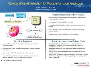
3. Given: protein sequence, knockout phenotype, gene expression profile, protein-protein interactions, and phylogenetic profile Predict a probability for every term in the Gene Ontology The problem • Heterogeneous data • Missing data • Multiple labels per gene • Structured output

4. Consistent predictions The probability that protein X is a cytoplasmic membrane-bound vesicle must be less than or equal to the probability that protein X is a cytoplasmic vesicle. Cytoplasmic membrane-bound vesicle (GO:0016023) is a Cytoplasmic vesicle (GO:0031410)

5. Data sets

7. Kernels

8. Gaussian Asymmetric Laplace SVM → Naïve Bayes Data 1 SVM/AL 1 Probability 1 Data 2 SVM/AL 2 Probability 2 Data 3 SVM/AL 3 Probability 3 Data 4 SVM/AL 4 Probability 4 Product, plus Bayes’ rule Data 5 SVM/AL 5 Probability Data 6 SVM/AL 6 Probability 6 Data 7 SVM/AL 7 Data 8 SVM/AL 8 Probability 8 Data 33 SVM/AL 33 Probability 33

9. SVM → logistic regression Data 1 SVM 1 Predict 1 Logistic regressor 1 Data 2 SVM 2 Predict 2 Data 3 SVM 3 Predict 3 Logistic regressor 2 Data 4 SVM 4 Predict 4 Logistic regressor 3 Data 5 SVM 5 Probability Data 6 SVM 6 Predict 6 Data 7 SVM 7 Data 8 SVM 8 Predict 8 Logistic regressor 11 Data 33 SVM 33 Predict 33

10. Reconciliation Methods • 3 heuristic methods • 3 Bayesian networks • 1 cascaded logistic regression • 3 projection methods

11. Heuristic methods • Max: Report the maximum probability of self and all descendants. • And: Report the product of probabilities of all ancestors and self. • Or: Compute the probability that at least one descendant of the GO term is “on,” assuming independence. • All three methods use probabilities estimated by logistic regression.

12. Bayesian network • Belief propagation on a graphical model with the topology of the GO. • Given Yi, the distribution of each SVM output Xi is modeled as an independent asymmetric Laplace distribution. • Solved using a variational inference algorithm. • “Flipped” variant: reverse the directionality of edges in the graph.

13. Cascaded logistic regression • Fit a logistic regression to the SVM output only for those proteins that belong to all parent terms. • Models the conditional distribution of the term, given all parents. • The final probability is the product of these conditionals:

14. Isotonic regression • Consider the squared Euclidean distance between two sets of probabilities. • Find the closest set of probabilities to the logistic regression values that satisfy all the inequality constraints.

15. Isotonic regression • Consider the squared Euclidean distance between two sets of probabilities. • Find the closest set of probabilities to the logistic regression values that satisfy all the inequality constraints.

16. Küllback-Leibler projection • Küllback-Leibler projection on the set of distributions which factorize according to the ontology graph. • Two variants, depending on the directions of the edges.

17. Hybrid method KLP BPAL BPLR Likelihood ratios obtained from logistic regression • Replace the Bayesian log posterior for Yiby the marginal log posterior obtained from the logistic regression. • Uses discriminative posteriors from logistic regression, but still uses a structural prior.

18. Ontology biological process cellular compartment molecular function Term size 3-10 proteins 11-30 proteins 31-100 proteins 100-200 proteins Evaluation mode Joint evaluation Per protein Per term Recall 1% 10% 50% 80% Axes of evaluation

19. Legend Belief propagation, asymmetric Laplace Belief propagation, asymmetric Laplace, flipped Belief propagation, logistic regression Cascaded logistic regression Isotonic regression Logistic regression Küllback-Leibler projection Küllback-Leibler projection, flipped Naïve Bayes, asymmetric Laplace

20. Joint evaluation Biological process ontology Large terms (101-200) Precision TP/(TP+FP) Recall TP / (TP+FN)

21. Biological process ontology

22. Molecular function ontology

23. Cellular compartment ontology

24. Conclusions: Joint evaluation • Reconciliation does not always help. • Isotonic regression performs well overall, especially for recall > 20%. • For lower recall values, both Küllback-Leibler projection methods work well.

25. Average precision per protein Biological process All term sizes

26. Biological process

27. Statistical significance Biological process Large terms

28. Biological process Large terms

29. Biological process 953 proteins 3-10 435 proteins 11-30 239 proteins 31-100 100 proteins 101-200

30. Molecular function 476 proteins 3-10 142 proteins 11-30 111 proteins 31-100 35 proteins 101-200

31. 196 proteins Cellular component 3-10 135 proteins 11-30 171 proteins 31-100 278 proteins 101-200

32. Conclusions: per protein • Several methods perform well • Unreconciled logistic regression • Unreconciled naïve Bayes • Isotonic regression • Belief propagation with asymmetric Laplace • For small terms • For molecular function and biological process, we do not observe many significant differences. • For cellular components, belief propagation with logistic regression works well.

33. Average precision per term Biological process All term sizes

34. Biological process 953 terms 3-10 435 terms 11-30 239 terms 31-100 100 terms 101-200

35. Molecular function 476 terms 3-10 142 terms 11-30 111 terms 31-100 35 terms 101-200

36. Cellular component 152 terms 3-10 97 terms 11-30 48 terms 31-100 30 terms 101-200

37. Conclusions • Reconciliation does not always help. • Isotonic regression (IR) performs well overall. • For small biological process and molecular function terms, it is less clear that IR is one of the best methods.

38. Acknowledgments Guillaume Obozinski Charles Grant Michael Jordan • The mousefunc organizers • Tim Hughes • Lourdes Pena-Castillo • Fritz Roth • Gabriel Berriz • Frank Gibbons Gert Lanckriet

39. Per term for small terms Biological process Molecular function Cellular component