Introducing Real Options: Expansion, Timing, and Learning Options
110 likes | 134 Vues
Explore the concept of real options and how they differ from discounted cash flow analysis. Learn how to value expansion options, timing options, and learning options. Understand when to use option pricing models for real options.

Introducing Real Options: Expansion, Timing, and Learning Options
E N D
Presentation Transcript
WEMBA 2000 Real Options 26 Introducing Real Options What are Real Options? Expansion Options: Starsoft Inc. is considering expanding its internet software product lines to include web page design software. If it does so, this will open up further expansion opportunities in the future, since the infrastructure requirements for developing web design software will undoubtedly be applicable to other web-based applications. Timing Options: Maxwell Corp. has a 3-year contract that gives it the right to develop a silver mine. However, the current price of silver is too low for the project to have a positive NPV. Maxwell has the choice between selling the contract today for a known price, or retaining it and waiting to see whether the price of silver increases sufficiently to make the mining project worthwhile. Learning Options Pharmacure is evaluating whether to begin R&D on a newdrug for treating certain types of cancer. Throughout the R&D process, the company will learn more about the drug's potential, the likely market demand, and any negative side-effects. As they gain new information, they can use it to adjust their level of spending on development, testing, and marketing costs.
WEMBA 2000 Real Options 27 Introducing Real Options How do Real Options differ from a standard Discounted Cash Flow/Decision Tree analysis? Project 1: High-risk Project 2: Low-risk 180 135 0.5 0.5 PV? PV? 0.5 0.5 50 95 Risk-adjusted PV @ 20% = 1* (180 + 50) 2 (1.20) = 95.8 Risk-adjusted PV @ 8% = 1* (135 + 95) 2 (1.08) = 106.50 Both projects have the same expected rate of return: (180 + 50)/2 = (135+95)/2 = 115 But…the variance in Project 1 is higher, hence we discount it at a higher rate. Now…suppose we have an option to exit either project in the "bad" scenario, in which case we would earn a salvage value of 110. How much would we pay for this option in either case?
WEMBA 2000 Real Options 28 Introducing Real Options Assume we have an option to exit the project, with a salvage value of 110. What is the new PV using standard Discounted Cash Flow analysis? Project 1 Project 2 180 135 0.5 0.5 PV? PV? 0.5 0.5 110 110 Risk-adjusted PV @ 20% = 1* (180 +110) 2 (1.20) = 120.8 Risk-adjusted PV @ 8% = 1* (135 + 110) 2 (1.08) = 113.4 Now Project 1 has a higher PV: 120.8 - 113.4 = 7.4 What is wrong with this analysis? Should we still be using 20% as the discount rate for Project 1? If not, what discount rate should we use?
WEMBA 2000 Real Options 29 Flashback to Binomial Pricing Methodology 2 Remember in Binomial Pricing Method 2 we calculated the “risk-neutral probability” as follows: Stock Price Option Value 22 1 q q 20 0.59 1-q 1-q 18 0 Call price = 0.59 = [1 * q + 0 * (1 - q)]/1.02 q = 0.6 Stock price = 20 = [22 * q + 18 * (1 - q)]/1.02 q = 0.6 We can use this technique to price real options very quickly! Step 1: calculate the risk-neutral probability from the stock price tree Step 2: calculate the option price using the risk-neutral probability
WEMBA 2000 Real Options 30 Using the Risk-Neutral Probability to price the Salvage Option in Project 1 Valuing the salvage option in Project 1 Project 1 without the salvage option Stock Price Option Value 180 max[0,K-S] = 0 q q 95.8 ?PV 1-q 1-q max[0, K-S] =60 50 Step 1: Solve for q (the “risk-neutral” probability) Step 2: Calculate the salvage option value using the risk-neutral probability Stock Price = 95.8 = [180*q + 50*(1 - q)]/1.05 q = 0.39 Put option = [0*q + 60*(1-q)]/(1.05) = [ 0*0.39 + 60*0.61]/(1.05) = 34.9 put = 34.9 Project Value = Project without the option + value of the option = 95.8 + 34.9 = 130.7
WEMBA 2000 Real Options 31 Using the Risk-Neutral Probability to price the Salvage Option in Project 2 Valuing the salvage option in Project 2 Project 2 without the salvage option Stock Price Option Value 135 max[0,K-S] = 0 q q 106.50 ?PV 1-q 1-q max[0, K-S] =15 95 Step 1: Solve for q (the “risk-neutral” probability) Step 2: Calculate the salvage option value using the risk-neutral probability Stock Price = 106.50 = [135*q + 95*(1 - q)]/1.05 q = 0.42 Put option = [0*q + 60*(1-q)]/(1.05) = [ 0*0.42 + 15*0.58]/(1.05) = 34.9 put = 8.3 Project Value = Project without the option + value of the option = 106.5 + 8.3 = 114.8
WEMBA 2000 Real Options 32 Introducing Real Options Project 1 Project 2 Difference PV using DCF analysis 120.8 113.4 7.4 PV using real options analysis: Project value without put 95.8 106.5 Put value 34.9 8.3 TOTAL 130.7 114.8 15.9 Using Discounted Cash Flow analysis, Project 1 is worth 7.4 more than Project 2 Using Binomial Option Pricing, Project 1 is worth 15.9 more than Project 2 Why is this the case? Options account for differing levels of risk at different times/scenarios (DCF uses the same discount rate throughout--which implies the same level of risk throughout) When can we use option pricing models for real options? When we can create a replicating portfolio of traded assets to neutralize the risk from the project
WEMBA 2000 Real Options 33 Case Study 1: Martha's Brewery, a micro-brewery startup Discounted Cash Flow analysis: Startup investment requirement: $4 million today Market launch: $12 million in two years time Today's NPV (based on projected cash flows) = -0.14 MM Reject Contingency plan: Market launch in two years only if market conditions are favorable Complication: How to evaluate the "option to expand"? Solution: Use option analysis to calculate present value of option to expand If present value of option less today's $4MM investment is positive: Accept!
WEMBA 2000 Real Options 34 Case Study 1: Martha's Brewery, a micro-brewery startup Discounted cash flow analysis: NPV = - 4 - 12 + 3.5 = - 0.14 (1.21) (1.21)(0.21) 6 3.5 Sales . . . earnings Time (years) 4 Cost of Capital Calculation: CAPM: E[r] = rf + (E[rm] - rf) = 5% + 2 * 8% = 21% 12
WEMBA 2000 Real Options 35 Case Study 1: Martha's Brewery, a micro-brewery startup Option analysis: Spot Price: Strike Price: Volatility: Expiration (years): Riskless rate: Call Value Option-adjusted Present value: 15 [Market-value-to-sales ratio for established micro-breweries = 3.66 Projected annual sales = 6 Spot price = 6 * 3.66 = 22 PV(Spot) = 15] 12 [Cost of follow-on investment if market conditions are favorable] 45% [from comparables] 1 [time at which $12 investment will be made if conditions are favorable] 5% 4.55 0.55 [4.55 - 4]
WEMBA 2000 Real Options 36 Case Study 1: Martha's Brewery, a micro-brewery startup Critical Assumptions for Option analysis: 1. Is spot price calculation realistic? Confidence in the sales estimate Use of market-value-to-sales ratio Alternative comparable analysis? (e.g. P/E ratio) 2. Is the current estimate of follow-on investment subject to change? 3. How was the implied volatility calculated? -- using historic volatility -- using existing options on publicly-traded micro-brewery companies 4. Riskless rate: which rate was used? 5. How confident are we about the timing of the follow-on investment?