Multiple alignment by aligning alignments
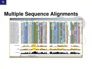
Multiple alignment by aligning alignments. Travis Wheeler John Kececioglu Department of Computer Science University of Arizona. Extended from talk given at ISMB ‘07. Multiple sequence alignment. Sequence alignment central to computational biology: Functional conservation

Multiple alignment by aligning alignments
E N D
Presentation Transcript
Multiple alignment by aligning alignments Travis Wheeler John Kececioglu Department of Computer Science University of Arizona Extended from talk given at ISMB ‘07
Multiple sequence alignment Sequence alignment central to computational biology: • Functional conservation • Phylogenetic analysis • Signals of selection • Prediction of structure • Comparative genomics • and many others …
Aligning two sequences A two-sequencealignment, with affine gap-costs, is scored, ) +l( ) )+ ( ( number of gaps substitution score total gap length columns g + 11 l ... ... g + 7 l g + 3 l
Scoring a multiple alignment Sum-of-pairs: wi,j score( i, j’ ) score( i, j” ) score( i, j ) i,j ij i j’ i j” ... Optimal alignment of multiple sequences is NP-complete Carrillo, Lipman 1988
Form-and-polish strategy • Choosing parameters • Constructing the merge tree • Grouping sequences • Measuring distances • Weighting sequence pairs • Merging alignments • Polishing the alignment
Form-and-polish strategy • Choosing parameters • Constructing the merge tree • Grouping sequences • Measuring distances • Weighting sequence pairs • Merging alignments • Polishing the alignment
Constructing merge tree gatac gacagg aacctacg aagccgtt aattt aatccgtt catccgtt Feng, Doolittle 1987
Merging alignments gatac gacagg aacctacg aagccgtt aattt aatccgtt catccgtt Feng, Doolittle 1987
gatac- gacagg aagccgtt aa---ttt aatccgtt catccgtt Merging alignments gatac gacagg aacctacg aagccgtt aattt aatccgtt catccgtt Feng, Doolittle 1987
aagccgtt aagccgtt aagccgtt aagccgtt aa---ttt aa---ttt aa---ttt aa---ttt aatccgtt aatccgtt catccgtt catccgtt aatccgtt catccgtt Merging alignments
A’ B’ Polishing the alignment • Split alignment into groups • Realign groups • Repeat A C B Berger, Munson 1991
Summary of main stages • Construct tree • Merge alignments • Polish
? Alignment Quality Computed alignment Correct alignment # substitutions recovered SPS : # substitutions in correct alignment # columns correctly recovered TC : # columns in correct alignment
Benchmark datasets • Benchmark suites • BAliBase [Thompson et al. 1999; Bahr et al. 2001] • PALI [Balaji et al 2001] • SABmark [Van Walle et al 2004] • All based on structural alignment of proteins • Characteristics • 900 alignments • 10 sequences per alignment, on average • 400 columns per alignment, on average • Core blocks • Regions with high support
Form-and-polish review • Choosing parameters • Constructing the merge tree • Grouping sequences • Measuring distances • Weighting sequence pairs • Merging alignments • Polishing the alignment
Grouping methods • Neighbor joining (NJ) [Saitou, Nei 1987] • Unweighted-pair group method with arithmetic mean (UPGMA) [Sneath, Sokal 1973] • Minimum spanning tree (MST) • Dynamic alignment distance (DAD)
Grouping sequences gacagg gatac aacctacg aatccgtt aagccgtt catccgtt aattt • Methods differ in measuring distances for new groups
Comparing grouping methods • Best grouping method ≠ best phylogeny method
Form-and-polish review • Choosing parameters • Constructing the merge tree • Grouping sequences • Measuring distances • Weighting sequence pairs • Merging alignments • Polishing the alignment
AHDHHSSQ AHDHHSSQ AHDHHSSQ AHDHHSSQ ANEH--TR ANEH--TR ANEH--TR ANEH--TR Measuring distances Percent identity Compressed identity Normalized alignment cost
Comparing distance methods • Normalized cost is very simple, and gives greatest gains
Form-and-polish review • Choosing parameters • Constructing the merge tree • Grouping sequences • Measuring distances • Weighting sequence pairs • Merging alignments • Polishing the alignment
) +l( )+ ( ( ) gap length substitution score columns ) ( wi,j i,j Aligning alignments gap count gap count
Merging methods Exact gap counts [Gotoh 1993 ; Kececioglu, Starrett 2004] • k sequences, n columns • O(5kn2) worst case • O(k2n2) time in practice Pessimistic gap counts [Altschul 1989; Kececioglu, Zhang 1998] • Overestimates gap startups • O(kn + n2) worst case • 100-fold speedup with 20 sequences per alignment
Comparing merging methods • Pessimistic heuristic may be sufficient for large inputs
Form-and-polish review • Choosing parameters • Constructing the merge tree • Grouping sequences • Measuring distances • Weighting sequence pairs • Merging alignments • Polishing the alignment
Polishing methods Two-cut method • Random partition [Probcons Do et al. 2005] • Tree-based partition
Polishing methods Two-cut method • Random partition [Probcons Do et al. 2005] • Tree-based partition • Randomly cut edges [MAFFT Katoh et al. 2005] • Exhaustively cut edges [Muscle Edgar 2004] • Can’t fix two small misaligned groups
Polishing methods Two-cut method • Random partition [Probcons Do et al. 2005] • Tree-based partition • Randomly cut edges [MAFFT Katoh et al. 2005] • Exhaustively cut edges [Muscle Edgar 2004] • Can’t fix two small misaligned groups
Polishing methods Two-cut method • Random partition [Probcons Do et al. 2005] • Tree-based partition • Randomly cut edges [MAFFT Katoh et al. 2005] • Exhaustively cut edges [Muscle Edgar 2004] • Can’t fix two small misaligned groups
Polishing methods Two-cut method • Random partition [Probcons Do et al. 2005] • Tree-based partition • Randomly cut edges [MAFFT Katoh et al. 2005] • Exhaustively cut edges [Muscle Edgar 2004] • Can’t fix two small misaligned groups Three-cut method • Tree-based, random
Polishing methods Two-cut method • Random partition [Probcons Do et al. 2005] • Tree-based partition • Randomly cut edges [MAFFT Katoh et al. 2005] • Exhaustively cut edges [Muscle Edgar 2004] • Can’t fix two small misaligned groups Three-cut method • Tree-based, random On-the-fly method [Subbiah, Harrison 1989]
Comparing polishing methods • 3-cut achieves 2-cut quality in less time • On-the-fly speeds up 2-cut convergence
Form-and-polish review • Choosing parameters • Constructing the merge tree • Grouping sequences • Measuring distances • Weighting sequence pairs • Merging alignments • Polishing the alignment
Weighting sequence pairs A B C 20 seqs 2 seqs 50 seqs
Weighting sequence pairs A 40 A-B pair alignments (20) 1000 A-C pair alignments B (2) 100 B-C pair alignments C (50)
Weighting methods Covariance weights [Altschul, et al. 1989] • Based on correlation between paths • Approximated in practice [Gotoh 1995] • Used in MAFFT Division weights [Thompson, et al. 1994] • Edge lengths divided among leaves • Used in ClustalW, Muscle
Weighting anomalies Covariance weights i if lvx 2 lvy = lvz then wyz 2wxz ≈ even for very long lvz wyz wxz (expect: ) ≈ v lvy lvx y z x
Weighting anomalies Division weights i if lvx lvy << lvz = lvz then wxz wyz 2wxy = ≈ wxy wxz wyz (expect: = ) ≈ 2lvz v lvx lvy x y z
Weighting methods Covariance weights [Altschul, et al. 1989] • Based on correlation between paths • Approximated in practice [Gotoh 1995] • Used in MAFFT Division weights [Thompson, et al. 1994] • Edge lengths divided among leaves • Used in ClustalW, Muscle Influence weights • Based on the influence of leaf j on i, i,j
Influence weights B A C j i
Influence weights i A’ A” B C j
Influence weights i x y z
Sx(y) : l(x,y) + ( l(e) ) e T(y) Sx(y) Nx(y) = Hx(y) Hx(y) Influence weights T(y) : tree under y (subtree) i (size) L(y) : set of leaves under y (leaf set) Hx(y) : avg path length from x to L(y) (height) x (effective # sequences) y z
Sx(y) : l(x,y) + ( l(e) ) e T(y) Sx(y) y Nx(y) = Hx(y) y Influence weights T(y) : tree under y (subtree) i (size) L(y) : set of leaves under y (leaf set) Hx(y) : avg path length from x to L(y) (height) x (effective # sequences) z Nx(y) ≈ 1 Nx(y) ≈ k k seqs
Sx(y) : l(x,y) + ( l(e) ) e T(y) Sx(y) Nx(y) = Hx(y) wy Nx(y) Hi(z) = wz Nx(z) Hi(y) Influence weights T(y) : tree under y (subtree) i (size) L(y) : set of leaves under y (leaf set) Hx(y) : avg path length from x to L(y) (height) wx x (effective # sequences) y z Split wx = wy + wz according to the ratio:
Sx(y) : l(x,y) + ( l(e) ) e T(y) 7 1 Sx(y) wx wx y Nx(y) = 8 8 Hx(y) wy Nx(y) Hi(z) = z wz Nx(z) Hi(y) Influence weights T(y) : tree under y (subtree) i (size) L(y) : set of leaves under y (leaf set) Hx(y) : avg path length from x to L(y) (height) wx x Hi(y) ≈ Hi(z) (effective # sequences) Split wx = wy + wz according to the ratio: Nx(z) ≈ 1 Nx(y) ≈ 7
Sx(y) : l(x,y) + ( l(e) ) e T(y) 2 1 Sx(y) wx wx Nx(y) = 3 3 Hx(y) wy Nx(y) Hi(z) = wz Nx(z) Hi(y) Nx(y) ≈ Nx(z) Influence weights T(y) : tree under y (subtree) i (size) wx L(y) : set of leaves under y (leaf set) x Hx(y) : avg path length from x to L(y) (height) y z (effective # sequences) Hi(y) = 5 Hi(z) = 10 Split wx = wy + wz according to the ratio:
Define wij = w(i,j) w(j,i) wi,j score( i, j ) i,j Influence weights • Influence w(i,j) is the weight wj SP score =

