Leveling
Leveling. Chapter 4. Why do we perform leveling surveys?. To determine the topography of sites for design projects Set grades and elevations for construction projects Compute volumes of earthwork. Old Datum: Mean Sea Level. Mean Sea Level (MSL) Average height over a 19-year period

Leveling
E N D
Presentation Transcript
Leveling Chapter 4
Why do we perform leveling surveys? • To determine the topography of sites for design projects • Set grades and elevations for construction projects • Compute volumes of earthwork
Old Datum: Mean Sea Level • Mean Sea Level (MSL) • Average height over a 19-year period • 26 gauging stations along the Atlantic Ocean, Pacific Ocean and the Gulf of Mexico
New Datum: NGVD88 • National Geodetic Vertical Datum of 1988 (NGVD88) • Completed in 1991, refined 1929 survey • Included 625,000 km of additional leveling • Single tidal gauge bench mark located in Quebec, Canada • Tidal gauge bench called Father Point/Rimouski
Effects of Curvature and Refraction The earth’s curvature causes a rod reading taken at point B to be too high. The effect of refraction is to make objects appear higher than they really are thus making the rod readings too low.
Curvature Equations Cf = 0.667 M2 = 0.0239 F2 (in feet)(U.S. Customary Units) And Cm = 0.0785 K2 (in meters) (Metric Units) Where: M – distance in miles F- distance in thousands of feet K – distance in kilometers
Refraction Equations Rf = 0.093 M2 = 0.0033 F2 (in feet)(U.S. Customary Units) And Rm = 0.011 K2 (in meters) (Metric Units) Where: M – distance in miles F- distance in thousands of feet K – distance in kilometers The refraction correction is about one-seventh the effect of curvature but in the opposite direction.
Combined Equations hf = 0.574 M2 = 0.0206 F2 (in feet)(U.S. Customary Units) and hm = 0.0675 K2 (in meters) (Metric Units) where: M – distance in miles F - distance in thousands of feet K – distance in kilometers
Effects of Curvature and Refraction For 300’ shot: hf = 0.0206 (300/1000)2 = 0.0019’ For 1000’ shot: hf = 0.0206 (1000/1000)2 = 0.0206’ Under the most adverse conditions (very hot humid conditions) the error associated with refraction can be as high as 0.10’ for a 200-foot shot.
Eliminating Effects of Curvature and Refraction Proper field procedures (taking shorter shots and balancing shots) can practically eliminate errors due to curvature and refraction.
Trigonometric Leveling Used in areas of very steep or rugged terrain or when you have inaccessible points.
Equations: If S and the vertical angle are determined: V = S sin or V = S cos z If H and the vertical angle are determined: V = H tan or V = H tan z The change in elevation between points A and B is: elev = hi + V – r where: hi – height of the instrument above point A
Equations (continued): and: r – rod reading at B when the vertical angle is read If r is made equal to the hi, then the two values cancel and the computations are simplified. These equations are applicable when shots are taken at less than 1000 feet. For shots longer than 1000 feet, the effects of curvature and refraction must be taken into account.
Equations: elev = hi + V + (C – R) – r where: (C –R) is computed from the equation: 0.0206 F2 See Example 4-1 on page 82 and Example 4-2 on page 83.