Download
1 / 95
1.07k likes | 1.52k Vues
Minimization or Maximization of Functions (Readings – 10.0 – 10.7 of NRC). Optimisation Methods. Introduction. You are given a single function f that depends on one or more independent variables. You want to find the value of those variables where f takes on a maximum or a minimum value.

E N D
Minimization or Maximization of Functions(Readings – 10.0 – 10.7 of NRC) Optimisation Methods
Introduction • You are given a single function f that depends on one or more independent variables. You want to find the value of those variables where f takes on a maximum or a minimum value. • An extremum (maximum or minimum point) can be either global (truly the highest or lowest function value) or local (the highest or lowest in a finite neighborhood and not on the boundary of that neighborhood). • The unconstrained multi-variable problem is written as min f(x) x RN where x is a vector of the decision variables.
Introduction Extrema of a function in an interval. Points A, C, and E are local, but not global maxima. Points B and F are local, but not global minima. The global maximum occurs at G, which is on the boundary of the interval so that the derivative of the function need not vanish there. The global minimum is at D. At point E, derivatives higher than the first vanish, a situation which can cause difficulty for some algorithms. The points X, Y , and Z are said to “bracket” the minimum F , since Y is less than both X and Z.
Contour Plots A contour plot consists of contour lines where each contour line indicates a specific value of the functionf(x1,x2).
Solution Methods • The solution methods are classified into 3 broad categories: • Direct (zero order) search methods: • Bisection Search • Golden Section Search • Parabolic Interpolation and Brent’s Method • Simplex Method • Powell’s Method • Gradient based (first order) methods: • Steepest descent • Conjugate gradient • Second order methods: • Newton • Modified Newton • Quasi-Newton
Direct(zero order) search methods They require only function values. The are computationally uncomplicated. They are slow.
How Small is Tolerably Small • (1-ε)b < b < (1 + ε)b where ε is computers precision (3 x 10⁻⁸ for single and 10-15 for double precision) • But: f(x) near b is (Taylor’s Theorem) is • The second term is negligible compared to the first when • Which is 3 x 10⁻⁴ for single and 10-8 for double precision
Bisection Method for Finding Roots of a Function • Bisection method : finds roots of functions in one dimension. The root is supposed to have been bracketed in an interval (a,b). • Evaluate the function at an intermediate point x and obtain a new, smaller bracketing interval, either (a,x) or (x,b). • The process continues until the bracketing interval is acceptably small. • It is optimal to choose x to be the midpoint of (a,b) so that the decrease in the interval length is maximized when the function is as uncooperative as it can be, i.e., when the luck of the draw forces you to take the bigger bisected segment.
Golden Section Search – 1D • Successive bracketing of a minimum. The minimum is originally bracketed by points 1,3,2. The function is evaluated at 4, which replaces 2; then at 5, which replaces 1; then at 6, which replaces 4. The rule at each stage is to keep a center point that is lower than the two outside points. After the steps shown, the minimum is bracketed by points 5,3,6.
Golden Section Search – Discussion 1 • New search interval will be either between x1 and x4 with a length of a+c , or between x2 and x3 with a length of b • To ensure that b = a+c, the algorithm should choose x4 = x1 − x2 + x3. • Question of where x2 should be placed in relation to x1 and x3. • The golden section search chooses the spacing between these points in such a way that these points have the same proportion of spacing as the subsequent triple x1,x2,x4 or x2,x4,x3. • By maintaining the same proportion of spacing throughout the algorithm, we avoid a situation in which x2 is very close to x1 or x3, and guarantee that the interval width shrinks by the same constant proportion in each step.
Golden Section Search – Discussion 1 • Mathematically, to ensure that the spacing after evaluating f(x4) is proportional to the spacing prior to that evaluation, if f(x4) is f4a and our new triplet of points is x1, x2, and x4 then we want c/a = a/b. • However, if f(x4) is f4b and our new triplet of points is x2, x4, and x3 then we want c/(b-c) = a/b • Eliminating c from these two simultaneous equations yields (b/a)2=(b/a)+1 and solving gives b/a = φ, the golden ratio, where:
Golden Section Search – Discussion 2 • Given (a,b,c), suppose b is a fraction w between a and c and the next trial point x is an additional fraction z between a and c. • The next bracketing segment will either be of length w + z or of length 1 – w. To minimise the worst case possibility these should be equal giving • Scale similarity implies that x should be the same fraction in b to c as b was in a to c giving: • Solving these gives w = 0.38197, the golden mean / section
Parabolic Interpolation • The Golden Section Search is designed to handle the worse possible case of function minimisation where the function has erratic behaviour • However most functions, if they are sufficiently smooth, are nearly parabolic near a minima. • Given three points near a minima, successively fitting a parabola to these three points should help to get a point closer to the minimum.
Parabolic Interpolation and Brent’s Method • The formula for x at the minimum of a parabola through three points f(a), f(b) and f(c) is:
Parabolic Interpolation and Brent’s Method • The exacting task is to invent a scheme that relies on a sure-but-slow technique, like golden section search, when the function is not cooperative, but that switches over to parabolic interpolation when the function allows. • The task is nontrivial for several reasons, including these: • The housekeeping needed to avoid unnecessary function evaluations in switching between the two methods can be complicated. • Careful attention must be given to the “endgame,” where the function is being evaluated very near to the round-off limit. • The scheme for detecting a cooperative versus non-cooperative function must be very robust.
Brent’s Method • Keeps track of 6 function points: • a and b bracket the minimum • Least function value found is at x • Second least function value at w • v is the previous value of w • u is the point at which function most recently evaluated • Parabolic interpolation is attempted fitting through x, v and w. • To be acceptable, the parabolic step must be between a and b, and imply a movement from x that is less than half the movement of the step before. • Where this is not working Brent’s Method alternates between parabolic steps and golden sections.
Brent’s Method with First Derivatives • First derivatives can be used within Brent’s Method as follows: The sign of the derivative at the central point of the bracketing triplet (a,b,c) indicates uniquely whether the next test point should be taken in the interval (a,b) or in the interval (b,c). The value of this derivative and of the derivative at the second-best-so-far point are extrapolated to zero by the secant method (inverse linear interpolation). • We impose the same sort of restrictions on this new trial point as in Brent’s method. If the trial point must be rejected, we bisect the interval under scrutiny.
Downhill Simplex Method in Multi-Dimensions • Bisection Methods only work in one dimension, • The downhill simplex method handles multi-dimensional problems and is due to Nelder and Mead. The method requires only function evaluations, not derivatives. • A simplex is the geometrical figure consisting, in N dimensions, of N +1 points (or vertices) and all their interconnecting line segments, polygonal faces, etc. • In two dimensions, a simplex is a triangle. In three dimensions it is a tetrahedron, not necessarily the regular tetrahedron.
Downhill Simplex Method in Multi-Dimensions • After initialisation, the downhill simplex method takes a series of steps, most steps just moving the point of the simplex where the function is largest through the opposite face of the simplex to a lower point. These steps are called reflections, and they are constructed to conserve the volume of the simplex (hence maintain its non-degeneracy). • When it can do so, the method expands the simplex in one or another direction to take larger steps. • When it reaches a “valley floor,” the method contracts itself in the transverse direction and tries to ooze down the valley. • If the simplex is trying to “pass through the eye of a needle,” it contracts itself in all directions, pulling itself in around its lowest (best) point.
Downhill Simplex Method in Multi-Dimensions • Let xi be the location of the ith vertex, ordered f(x1)>f(x2)…>f(xD+1). • Center of face of the simplex defined by all vertices other than the one we are trying to improve, • Since all of the others have a better function value, they give a good direction to move in; reflection
Downhill Simplex Method in Multi-Dimensions • If a new position is better, it is worth checking to see if it’s even better to double the size of the step; expansion • If a new position is worse, it means we overshot. Then, reflect andshrink
Downhill Simplex Method in Multi-Dimensions • If after reflecting and shrinking a new position is still worse, we can try just shrinking; • If after shrinking a new position is still worse, give up and shrink all of the vertices towards the best one • When it reaches a minimum it will give up and shrink down around it, triggering a stopping decision when the values are no longer improving.
Downhill Simplex Method in Multi-Dimensions Solve by applying 5 iterations of the simplex method, starting with x0 = [5, 2]T. (5, 2) f = 234
Downhill Simplex Method in Multi-Dimensions Iteration 1 (5.51, 4.63) f = 576.31 (6.8, 4.12) f = 851.91 (5, 2) f = 234
Downhill Simplex Method in Multi-Dimensions Iteration 2 (5.51, 4.63) f = 576.31 (3.63, 2.51) f = 102.88 (5, 2) f = 234
Downhill Simplex Method in Multi-Dimensions Iteration 3 (3.63, 2.517) f = 102.88 (5, 2) f = 234 (3.12, -0.1204) f = 64.71
Downhill Simplex Method in Multi-Dimensions Iteration 4 (3.638, 2.517) f = 102.88 (1.75, 0.397) f = 5.15 (3.12, -0.1204) f = 64.71
Downhill Simplex Method in Multi-Dimensions Iteration 5 The solution (1.758, 0.3972) f = 5.51 (3.12, -0.12) f = 64.71 (1.24, -2.24) f = 61.877
Downhill Simplex Method in Multi-Dimensions Rosenbrock’s “banana” function F=100(x2-x12)2+(x1-1)2
Direction Set Methods General Scheme Initial Step set k = 0 supply an initial guess, xk, within any specified constraints Iterative Step calculate a search direction pk determine an appropriate step length lk set xk+1 to xk+ lk pk Stopping Criteria if convergence criteria reached optimum vector is xk+1 stop else set k = k + 1 repeat Iterative Step
Direction Set (Powell’s) Method • Sometimes it is not possible to estimate the derivative ∂f to obtain the direction in a steepest descent method • First guess, minimize along one coordinate axis, then along other and so on. Repeat • Can be very slow to converge Conjugate directions: Directions which are independent of each other so that minimizing along each one does not move away from the minimum in the other directions. Powell introduced a method to obtain conjugate directions without computing the derivative.
Direction Set (Powell’s) Method If f is minimised along u, then must be perpendicular to u at the minimum. The function may be expanded using the Taylor series around the origin p as: By taking the gradient of the Taylor expansion The change in gradient when moving in one direction is: After f is minimised alongu, the algorithm proposes a new direction v so that minimisation along v does not spoil the minimum along u. For this to be true, the function gradient must stay perpendicular to u When this is true, u and v are said to be conjugate and we get quadratic convergence to the minimum
Direction Set (Powell’s) Method • Initialise the set of directions ui to the basis vectors • Repeat until function stops decreasing: • Save starting position as P0 • For i = 0..N-1, movePito the minimum along direction ui and call this point Pi+1 • For i = 0..N-2, set ui = ui+1 • Set uN-1 = PN-P0 • Move PN to the minimum along direction uN-1 and call this point P0 Powell showed that, for a quadratic form, k iterations of the above procedure produce a set of directions ui whose last k members are mutually conjugate. Therefore, N iterations involving N(N+1) line minimisations will exactly minimise a quadratic form.
Gradient Based Methods They employ the gradient information. They are iterative methods and employ the iteration procedure • where (k) : step size • s(x(k)): direction. The methods differ in how s(x(k)) is computed.
Steepest Descent Method • Let x(k) be the current point. • The Taylor expansion of the objective function about x(k): • We need the next point to have a lower objective function value than the current point: • That is equivalent to • The smallest value of this product is when
Steepest Descent Method • We call this direction the steepest descent direction. • Another proof of the steepest descent direction is to recognize that the gradient always points towards increasing value of the objective function. • Taking the negative of the gradient, then, leads to the decreasing value of the objective function. • Now the direction is determined, a single variable search is needed to determine the value of the step size. • In every iteration of the method, the direction and step size are computed.
Steepest Descent Method • Notes • The good thing about the steepest descent method is that it always converges. • What’s bad about it is that it converges slower as the minimum is approached.
Steepest Descent Method • The gradient represents the perpendicular line to the tangent of the contour line of the function at a particular point.