The nonperturbative analyses for lower dimensional non-linear sigma models
240 likes | 427 Vues
The nonperturbative analyses for lower dimensional non-linear sigma models. 1.Introduction 2.The WRG equation for NLσM 3.Fixed points with U(N) symmetry 4.3-dimensional case 5. Summary. Etsuko Itou (Kanazawa University). 1. Introduction.

The nonperturbative analyses for lower dimensional non-linear sigma models
E N D
Presentation Transcript
The nonperturbative analyses for lower dimensional non-linear sigma models 1.Introduction 2.The WRG equation for NLσM 3.Fixed points with U(N) symmetry 4.3-dimensional case 5. Summary Etsuko Itou (Kanazawa University)
1. Introduction We consider the Wilsonian effective action which has derivative interactions. It corresponds to the non-linear sigma model action, so we compare the results with the perturbative one. It corresponds to next-to-leading order approximation in derivative expansion. Local potential term Non-linear sigma model Local potential approximation : K.Aoki Int.J.Mod.Phys. B14 (2000) 1249 T.R.Morris Int.J.Mod.Phys. A9 (1994) 2411
The point of view of non-linear sigma model: Two-dimensional case ●In perturbative analysis, the 1-loop b function for 2-dimensional non-linear sigma model proportional to Ricci tensor of target spaces. ⇒Ricci Flat Is there the other fixed point? The perturbative results Alvarez-Gaume, Freedman and Mukhi Ann. of Phys. 134 (1982) 392
Three-dimensional case ●The 3-dimensional non-linear sigma models are nonrenormalizable within the perturbative method. We need some nonperturbative renormalization methods. WRG approach Large-N expansion Inami, Saito and Yamamoto Prog. Theor. Phys. 103 (2000)1283
2.The WRG equation for NLσM The Euclidean path integral is K.Aoki Int.J.Mod.Phys. B14 (2000) 1249 The Wilsonian effective action has infinite number of interaction terms. The WRG equation (Wegner-Houghton equation) describes the variation of effective action when energy scale L is changed to L(dt)=L exp[-dt] .
To obtain the WRG eq. , we integrate shell mode. only The Wilsonian RG equation is written as follow: Field rescaling effects to normalize kinetic terms. We use the sharp cutoff equation. It corresponds to the sharp cutoff limit of Polchinski equation at least local potential level.
Approximation method: Symmetry and Derivative expansion Consider a single real scalar field theory that is invariant under We expand the most generic action as In this work, we expand the action up to second order in derivative and assume it =2 supersymmetry.
D=2 (3) N =2 supersymmetric non linear sigma model i=1~N:N is the dimensions of target spaces Where K is Kaehler potential and F is chiral superfield.
We expand the action around the scalar fields. where : the metric of target spaces From equation of motion, the auxiliary filed F can be vanished. Considering only Kaehler potential term corresponds to second order to derivative for scalar field. There is not local potential term.
The WRG equation for non linear sigma model Consider the bosonic part of the action. The second term of the right hand side vanishes in this approximation O( ) .
The first term of the right hand side From the bosonic part of the action From the fermionic kinetic term Non derivative term is cancelled.
Finally, we obtain the WRG eq. for bosonic part of the action as follow: The b function for the Kaehler metric is The perturbative results Alvarez-Gaume, Freedman and Mukhi Ann. of Phys. 134 (1982) 392
3. Fixed points with U(N) symmetry The perturbative βfunction follows the Ricci-flat target manifolds. Ricci-flat We derive the action of the conformal field theory corresponding to the fixed point of the b function. To simplify, we assume U(N) symmetry for Kaehler potential. where
The function f(x) have infinite number of coupling constants. The Kaehler potential gives the Kaehler metric and Ricci tensor as follows:
The solution of the β=0 equation satisfies the following equation: Here we introduce a parameter which corresponds to the anomalous dimension of the scalar fields as follows: When N=1, the function f(x) is givenin closed form The target manifold takes the form of a semi-infinite cigar with radius . It is embedded in 3-dimensional flat Euclidean spaces. Witten Phys.Rev.D44 (1991) 314
This solution has been discussed in other context. They consider the non-linear sigma model coupled with dilaton. Witten Phys.Rev.D44 (1991) 314 Kiritsis, Kounnas and Lust Int.J.Mod.Phys.A9 (1994) 1361 Hori and Kapustin :JHEP 08 (2001) 045 In k>>1 region, we can use the perturbative renormalization method and obtain 1-loop b function: If one prefers to stay on a flat world-sheet, one may say that a non-trivial dilaton gradient in space-time is equivalent to assigning a non-trivial Weyl transformation law to target space coordinates. Our parameter a (anomalous dim.) corresponds to k as follow.
4.3-dimensional case The 3-dimensional non-linear sigma models are nonrenormalizable within the perturbative method. We need some nonperturbative renormalization methods. Similarly to 2-dimenion, we obtain the nonperturbative b function for 3-dimensional non-linear sigma models.
When the target space is an Einstein-Kaehler manifold, the βfunction of the coupling constant is obtained. Einstein-Kaehler condition: If the constant h is positive, there are two fixed points: At UV fixed point
The CPNmodel :SU(N+1)/[SU(N) ×U(1)] If the constant h is positive, it is possible to take the continuum limit by choosing the cutoff dependence of the bare coupling constant as M is a finite mass scale.
We derive the action of the conformal field theory corresponding to the fixed point of the b function. To simplify, we assume SU(N) symmetry for Kaehler potential. We substitute the metric and Ricci tensor given by this Kaehler potential for following equation.
The following function satisfies b=0 for any values of parameter A free parameter, , is proportional to the anomalous dimension. If we fix the value of , we obtain a conformal field theory.
We take the specific values of the parameter, the function takes simple form. ● This theory is equal to IR fixed point of CPNmodel ● This theory is equal to UV fixed point of CPNmodel. Then the parameter describes a marginal deformation from the IR to UV fixed points of the CPNmodel in the theory spaces.
5. Summary In this work, we consider the derivative interaction terms using Wilsonian RG equation which has sharp cutoff. The RG flows for some concrete models agree with the perturbative or large-N results. We construct a class of fixed point theory for 2- and 3-dimensional supersymmetric NLσM. These theory has one free parameter which corresponds to the anomalous dimension of the scalar fields. In the 2-dimensional case, these theory coincide with perturbative 1-loop βfunction solution for NLσM coupled with dilaton. In the 3-dimensional case, the free parameter describes a marginal deformation from the IR to UV fixed points of the CPNmodel in the theory spaces.