MergeSort
240 likes | 471 Vues
MergeSort. Algorithm : Design & Analysis [7]. In the last class …. General pattern of divide-and conquer Quicksort: the Strategy Quicksort: the Algorithm Analysis of Quicksort Improvements of the Algorithm Average Behavior of Quicksort Guess and Proof

MergeSort
E N D
Presentation Transcript
MergeSort Algorithm : Design & Analysis [7]
In the last class… • General pattern of divide-and conquer • Quicksort: the Strategy • Quicksort: the Algorithm • Analysis of Quicksort • Improvements of the Algorithm • Average Behavior of Quicksort • Guess and Proof • Solving Recurrence Equation Directly
Mergesort • Mergesort • Worst Case Analysis of Mergesort • Lower Bounds for Sorting by Comparison of Keys • Worst Case • Average Behavior
Merging Sorted Arrays A[k-1] A[0] B[0] B[m-1]
Merge: the Specification • Input: Array A with k elements and B with m elements, each in nondecreasing order of their key. • Output: C, an array containing n=k+m elements from A and B in nondecreasing order. C is passed in and the algorithm fills it.
Merge: the Recursive Version merge(A,B,C) if (A is empty) rest of C = rest of B else if (B is empty) rest of C = rest of A else if (first of A first of B) first of C =first of A merge(rest of A, B, rest of C) else first of C =first of B merge(A, rest of B, rest of C) return Base cases
Merge: the Iterative Version void merge(Element [ ] A, intk, Element[ ] B, intm, Element[ ] C) intn=m+k; int indexA=0; indexB=0; indexC=0 // beginning of rest of A,B,C while (indexA<k && indexB<m) if A[indexA].key B[indexB].key C[indexC]=A[indexA]; indexA++; indexC++; else C[indexC]=B[indexB]; indexB++; indexC++; //continue loop if (indexAk) copy B[indexB, ..., m-1] to C[indexC, ..., n-1] else copy A[indexA, ..., m-1] to C[indexC, ..., n-1]
Worst Case Complexity of Merge • Observations: • After each comprison, one element is inserted into Array C, at least. • After entering Array C, an element will never be compared again • After the last comparison, at least two elements have not yet been moved to Array C. So at most n-1 comparisons are done. • Worst case is that the last comparison is conducted between A[k-1] and B[m-1] • In worst case, n-1 comparisons are done, where n=k+m
Optimality of Merge • Any algorithm to merge two sorted arrays, each containing k=m=n/2 entries, by comparison of keys, does at least n-1 comparisons in the worst case. • Choose keys so that: b0<a0<b1< a1<...<bi<ai<bi+1,...,<bm-1<ak-1 • Then the algorithm must compare ai with bi for every i in [0,m-1], and must compare ai with bi+1 for every i in [0, m-2], so, there are n-1 comparisons.
Optimality of Merge, with km • Any algorithm to merge two sorted arrays, by comparison of keys, where the inputs contain k and m entries, respectively, k and m differ at most by one, and n=k+m, does at least n-1such comparisons in the worst case.
Space Complexity of Merge • A algorithm is “in space”, if the extra space it has to use is in (1) • Merge is not a algorithm “in space”, since it need enough extra space to store the merged sequence during the merging process.
Looking back at Quicksort • Quicksort is not“in space”. • Space cost originated from recursion • Deep recursion results in low space efficiency
MergeSort: the Strategy • Easy division • No comparison is done during the division • Minimizing the size difference between the divided subproblems • Merging two sorted subranges • Using Merge
MergeSort • Input: Array E and indexes first, and last, such that the elements of E[i] are difined for firstilast. • Output: E[first],…,E[last] is a sorted rearrangement of the same elements. • Procedure voidmergeSort(Element[] E, int first, int last) if (first<last) int mid=(first+last)/2; mergeSort(E, first, mid); mergeSort(E, mid+1, last); merge(E, first, mid, last) return
Analysis of Mergesort • The recurrence equation for Mergesort • W(n)=W(n/2)+W(n/2)+n-1 • W(1)=0 Where n=last-first+1, the size of range to be sorted • The Master Theorem applies for the equation, so: W(n)(nlogn)
Recursion Tree for Mergesort n-1 Level 0 Base cases occur at depth lg(n+1)-1 and lg(n+1) Level 1 n-2 Level 2 n-4 n-8 Level 3 Note: nonrecursive costs on level k is n-2kfor all level without basecase node T(n) n-1 n/2-1 T(n/2) k/2 may be k/2 or k/2 n/8-1 T(n/8) T(n/4) n/4-1
Non-complete Recursive Tree Example: n=11 2D-1 nodes B base-case nodes on the second lowest level Since each nonbase-case node has 2 children, there are (n-B)/2 nonbase-case nodes at depth D-1 n-B base-case nodes No nonbase-case nodes at this depth
Number of Comparison of Mergesort • The maximum depth D of the recursive tree is lg(n+1). • Let B base case nodes on depth D-1, and n-B on depth D, (Note: base case node has nonrecursive cost 0). • (n-B)/2 nonbase case nodes at depth D-1, each has nonrecursive cost 1. • So: • nlg(n)-n+1 number of comparison nlg(n)-0.914n
Decision Tree for Sorting Internal node A example for n=3 • Decision tree is a 2-tree.(Assuming no same keys) • The action of Sort on a particular input corresponds to following on path in its decision tree from the root to a leaf associated to the specific output External node
Characteristics of the Decision Tree • For a sequence of n distinct elements, there are n! different permutation, so, the decision tree has at least n! leaves, and exactly n! leaves can be reached from the root. So, for the purpose of lower bounds evaluation, we use trees with exactly n! leaves. • The number of comparison done in the worst case is the height of the tree. • The average number of comparison done is the average of the lengths of all paths from the root to a leaf.
Lower Bound for Worst Case • Theorem: Any algorithm to sort n items by comparisons of keys must do at least lgn!, or approximately nlgn-1.443n, key comparisons in the worst case. • Note: Let L=n!, which is the number of leaves, then L2h, where h is the height of the tree, that is h lgL=lgn! • For the asymtotic behavior: derived using:
Lower Bound for Average Behavior • Since a decision tree with L leaves is a 2-tree, the average path length from the root to a leaf is . • The trees that minimize epl are as balanced as possible. • Recall that epl Llg(L). • Theorem: The average number of comparison done by an algorithm to sort n items by comparison of keys is at least lg(n!), which is about nlgn-1.443n.
Reducing External Path Length Assuming that h-k>1, when calculating epl, h+h+k is replaced by (h-1)+2(k+1). The net change in epl is k-h+1<0, that is, the epl decreases. X level k X level k +1 Y level h - 1 Y level h
Home Assignment • pp.212- • 4.25 • 4.27 • 4.29 • 4.30