Download
1 / 14
140 likes | 276 Vues
This research presents advanced methods for the simplification of point-sampled surfaces with an emphasis on maintaining the originality and characteristics of polygonal models. By reducing the polygon count while preserving essential surface properties, the techniques enhance computational efficiency. The study outlines point cloud clustering, iterative simplification, triangulation, and covariance analysis. Key approaches include local surface properties evaluation, region-growing clustering, and hierarchical clustering, aiming to optimize the rendering process without losing detail in the representation of complex models.

E N D
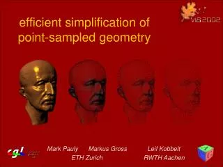
Efficient Simplification of Point-Sampled Surfaces CGIV, 16 March2006, Dongseo University Graduate School of Software Dongseo University, Busan Nam Woo Kim, d5302010@dongseo.ac.kr http://kowon.dongseo.ac.kr/~d5302010
Polygonal Simplification • Simplification is the method to deform polygonal model. • The objectives of simplification • Keeping the originality and characteristic of given models. • Reducing the number of polygons.
Outline Point cloud Clustering Iterative Simplification Triangulation
Local surface properties P1 P2 P3 P4 P5 P6
k k k P P P P ¡ r m a x = N i i i 2 ½ = p 2 r k -nearest neighbors r
T 0 1 0 1 ¡ ¡ p p p p i i n 1 1 1 N P P 3 3 £ X i ¡ ¡ p p p p p i i p p B C B C = i 2 2 C N i B C B C 2 n = j p ; . . B C B C i 1 = . . @ A @ A . . ¡ ¡ p p p p i i k k Covariance Analysis r Symmetric positive semi-definite matrix
f g ¸ ¸ ¸ l C N i 0 1 2 2 2 ¢ ¢ v p v v = l l l l l l i p ; ; ; ; Eigenalysis of covariance are real-valued eigenvectors from an orthogonal frame The measure the variation of the
( ) ¸ ¸ T P P v v x i 1 0 1 0 ¸ ( ) ( ) 0 ¸ ¸ ¸ T P 0 · · ¡ ( ) ¢ x : x v P = 0 1 2 0 ¾ = n ¸ ¸ ¸ + + 0 1 2 Normal Estimation Covariance ellipsoid
Clustering • Clustering by Region-growing • Hierarchical Clustering
C C C 0 1 2 Region-growing
BSP Tree in 2_Dimensional P P NULL
j j ( ) P P ¾ ¾ v n m a x 2 The size is larger than the user specified maximum cluster size or The variation is above a maximum threshold Hierarchical Clustering split plane leaf node =cluster centroid
P n 1 ( ) ( ) ¸ ¸ ¸ T P 0 · · ¡ X ¢ x : x v = 0 1 2 0 p p = i n i 1 = leaf node =cluster Iterative Simplification
Triangulation Voronoi diagram & Delaunay Triangulation’s Application