Understanding Multiple Regression Modeling in Economics
150 likes | 235 Vues
Learn about multiple regression modeling, endogenous variables, OLS estimator properties, measures of variation, calculating R2 values, standard error estimates, and the coefficient of determination. Explore examples and understand the significance of these concepts in economic analysis.

Understanding Multiple Regression Modeling in Economics
E N D
Presentation Transcript
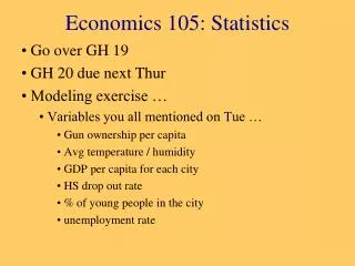
Economics 105: Statistics Go over GH 19 GH 20 due next Thur Modeling exercise … Variables you all mentioned on Tue … Gun ownership per capita Avg temperature / humidity GDP per capita for each city HS drop out rate % of young people in the city unemployment rate
The Multiple Regression Model Idea: Examine the linear relationship between 1 dependent (Y) & 2 or more independent variables (Xi) Multiple Regression Model with k Independent Variables: Population slopes Random Error Y-intercept • Endogenous explanatory variables
Modeling Exercise examples • What is the effect of your roommate’s SAT scores on your grades? The effect of studying? • Do police reduce crime? • Does more education increase wages? • What is the effect of school start time on academic achievement? • Does movie violence increase violent crime?
Endogenous Explanatory Variable • Causes of endogenous explanatory variables include … • Wrong functional form • Omitted variable bias … occurs if both the • Omitted variable theoretically determines Y • Omitted variable is correlated with an included X • Errors-in-variables (aka, measurement error) • Sample selection bias • Simultaneity bias (Y also determines X)
Unbiased estimator • Efficiency of an estimator • Intuition for when var is smaller • We won’t know , so we’ll need to estimate it Properties of OLS Estimator • Gauss-Markov Theorem • Under assumptions (1) - (5) [don’t need normality of errors], is B.L.U.E. of
Measures of Variation • Total variation is made up of two parts: Total Sum of Squares Regression Sum of Squares Error Sum of Squares where: = Average value of the dependent variable Yi = Observed values of the dependent variable i = Predicted value of Y for the given Xi value
Measures of Variation (continued) Y Yi Y SSE= (Yi-Yi)2 _ SST=(Yi-Y)2 _ Y _ SSR = (Yi -Y)2 _ Y Y X Xi
Goodness of Fit • The coefficient of determination is the portion of the total variation in Y that is explained by variation in X • Also called r-squared and denoted r2 (or R2)
Examples of Approximate R2 Values Y R2= 1 Perfect linear relationship between X and Y: 100% of the variation in Y is explained by variation in X X R2= 1 Y X R2= 1
Examples of Approximate R2Values Y 0 < R2< 1 Weaker linear relationships between X and Y: Some but not all of the variation in Y is explained by variation in X X Y X
Examples of Approximate R2Values R2= 0 Y No linear relationship between X and Y: The value of Y does not depend on X. (None of the variation in Y is explained by variation in X) X R2= 0
Standard Error of the Estimate • The variation of observations around the sample regression line is estimated by • an unbiased estimator of stddev of error term • where SSE = error sum of squares • n = sample size • K = number of slope beta parameters • Also called “standard error of the model,” or “root mean squared error” (RMSE). Book calls SYX.
Comparing Standard Errors • Seis a measure of the variation of observed Y values around the regression line Y Y X X • The magnitude of Seshould always be judged relative to the variation of the Y values in the sample data (measured by SY, the sample standard deviation of the actual Y values) • Closer to 0, than to sY , the better the fit
The coefficient of determination, , in simple regressions of the form, is equal to the square of the correlation coefficient. • Provides a link between correlation and regression • “Multiple R” is • In multiple regression context, • It is another, less commonly used, measure of strength of the relationship between the dependent var and the independent (explanatory) vars. “Multiple R”
Goodness of Fit • One should not place too much importance on obtaining a high R2 • If all else is equal, a model with a higher R2 explains a higher fraction of the variance • The model has more explanatory power • Dependent var must be the same to compare • However, R2 can be influenced by factors such as the nature of the data • Cross-sectional data on individual people: .1 to .2 • Cross-sectional data on firms, counties, cities, countries, states: .4 to .6 • Time-series data: > .80