Chapter 9: Trace Elements
Chapter 9: Trace Elements. Note magnitude of major element changes.

Chapter 9: Trace Elements
E N D
Presentation Transcript
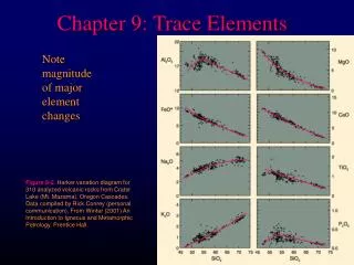
Chapter 9: Trace Elements Note magnitude of major element changes Figure 8-2.Harker variation diagram for 310 analyzed volcanic rocks from Crater Lake (Mt. Mazama), Oregon Cascades. Data compiled by Rick Conrey (personal communication).From Winter (2001) An Introduction to Igneous and Metamorphic Petrology. Prentice Hall.
Chapter 9: Trace Elements Now note magnitude of trace element changes Figure 9-1. Harker Diagram for Crater Lake. From data compiled by Rick Conrey. From Winter (2001) An Introduction to Igneous and Metamorphic Petrology. Prentice Hall.
Element Distribution Goldschmidt’s rules (simplistic, but useful) 1.2 ions with the same valence and radius should exchange easily and enter a solid solution in amounts equal to their overall proportions How does Rb behave? Ni?
Goldschmidt’s rules • 2. If 2 ions have a similar radius and the same valence: the smaller ion is preferentially incorporated into the solid over the liquid Fig. 6-10. Isobaric T-X phase diagram at atmospheric pressure After Bowen and Shairer (1932), Amer. J. Sci. 5th Ser., 24, 177-213. From Winter (2001) An Introduction to Igneous and Metamorphic Petrology. Prentice Hall.
3. If 2 ions have a similar radius, but different valence: the ion with the higher charge is preferentially incorporated into the solid over the liquid
Chemical Fractionation • The uneven distribution of an ion between two competing (equilibrium) phases
Exchange equilibrium of a componentibetween two phases (solid and liquid) i(liquid) = i(solid) eq. 9-2 K = = K =equilibrium constant Xsolid Xliquid a solid a liquid i i i i i i
Trace element concentrations are in the Henry’s Law region of concentration, so their activity varies in direct relation to their concentration in the system • Thus if XNi in the system doubles the XNi in all phases will double • This does not mean that XNi in all phases is the same, since trace elements do fractionate. Rather the XNi within each phase will vary in proportion to the system concentration
incompatible elements are concentrated in the melt (KD or D) « 1 • compatible elements are concentrated in the solid KD or D » 1
CS CL • For dilute solutions can substitute D for KD: D = Where CS = the concentration of some element in the solid phase
Incompatible elements commonly two subgroups • Smaller, highly charged high field strength (HFS)elements(REE, Th, U, Ce, Pb4+, Zr, Hf, Ti, Nb, Ta) • Low field strength large ion lithophile (LIL) elements (K, Rb, Cs, Ba, Pb2+, Sr, Eu2+) are more mobile, particularly if a fluid phase is involved
Compatibility depends on minerals and melts involved. Which are incompatible? Why?
eq. 9-4:Di = WA Di WA = weight % of mineral A in the rock Di = partition coefficient of element i in mineral A A A • For a rock, determine the bulk distribution coefficient D for an element by calculating the contribution for each mineral
Example: hypothetical garnet lherzolite = 60% olivine, 25% orthopyroxene, 10% clinopyroxene, and 5% garnet (all by weight), using the data in Table 9-1, is: DEr = (0.6 · 0.026) + (0.25 · 0.23) + (0.10 · 0.583) + (0.05 · 4.7) = 0.366
Trace elements strongly partitioned into a single mineral • Ni - olivine in Table 9-1 = 14 Figure 9-1a. Ni Harker Diagram for Crater Lake. From data compiled by Rick Conrey. From Winter (2001) An Introduction to Igneous and Metamorphic Petrology. Prentice Hall.
Incompatible trace elements concentrate liquid • Reflect the proportion of liquid at a given state of crystallization or melting Figure 9-1b. Zr Harker Diagram for Crater Lake. From data compiled by Rick Conrey. From Winter (2001) An Introduction to Igneous and Metamorphic Petrology. Prentice Hall.
Trace Element Behavior • The concentration of a major element in a phase is usually buffered by the system, so that it varies little in a phase as the system composition changes At a given T we could vary Xbulk from 35 70 % Mg/Fe without changing the composition of the melt or the olivine
Trace elementconcentrations are in the Henry’s Law region of concentration, so their activity varies in direct relation to their concentration in the system
Trace element concentrations are in the Henry’s Law region of concentration, so their activity varies in direct relation to their concentration in the system Thus if XNi in the system doubles the XNi in all phases will double
Trace element concentrations are in the Henry’s Law region of concentration, so their activity varies in direct relation to their concentration in the system Thus if XNi in the system doubles the XNi in all phases will double Because of this, the ratios of trace elements are often superior to the concentration of a single element in identifying the role of a specific mineral
K/Rb often used the importance of amphibole in a source rock • K & Rb behave very similarly, so K/Rb should be ~ constant • If amphibole, almost all K and Rb reside in it • Amphibole has a D of about 1.0 for K and 0.3 for Rb
Sr and Ba (also incompatible elements) • Sr is excluded from most common minerals except plagioclase • Ba similarly excluded except in alkali feldspar
Compatible example: • Ni strongly fractionated olivine > pyroxene • Cr and Scpyroxenes » olivine • Ni/Cr or Ni/Sc can distinguish the effects of olivine and augite in a partial melt or a suite of rocks produced by fractional crystallization
Models of Magma Evolution • Batch Melting • The melt remains resident until at some point it is released and moves upward • Equilibrium melting process with variable % melting
C 1 = L - + C Di (1 F) F O Models of Magma Evolution • Batch Melting eq. 9-5 CL = trace element concentration in the liquid CO = trace element concentration in the original rock before melting began F = wt fraction of melt produced = melt/(melt + rock)
Batch Melting A plot of CL/CO vs. F for various values of Di using eq. 9-5 • Di = 1.0 Figure 9-2. Variation in the relative concentration of a trace element in a liquid vs. source rock as a fiunction of D and the fraction melted, using equation (9-5) for equilibrium batch melting. From Winter (2001) An Introduction to Igneous and Metamorphic Petrology. Prentice Hall.
Di » 1.0 (compatible element) • Very low concentration in melt • Especially for low % melting (low F) Figure 9-2. Variation in the relative concentration of a trace element in a liquid vs. source rock as a fiunction of D and the fraction melted, using equation (9-5) for equilibrium batch melting. From Winter (2001) An Introduction to Igneous and Metamorphic Petrology. Prentice Hall.
Highly incompatible elements • Greatly concentrated in the initial small fraction of melt produced by partial melting • Subsequently diluted as F increases Figure 9-2. Variation in the relative concentration of a trace element in a liquid vs. source rock as a fiunction of D and the fraction melted, using equation (9-5) for equilibrium batch melting. From Winter (2001) An Introduction to Igneous and Metamorphic Petrology. Prentice Hall.
1 C L = - + C Di (1 F) F O • As F 1 the concentration of every trace element in the liquid = the source rock (CL/CO 1) As F 1 CL/CO 1 Figure 9-2. Variation in the relative concentration of a trace element in a liquid vs. source rock as a fiunction of D and the fraction melted, using equation (9-5) for equilibrium batch melting. From Winter (2001) An Introduction to Igneous and Metamorphic Petrology. Prentice Hall.
1 C L = - + C Di (1 F) F O As F 0 CL/CO 1/Di If we know CL of a magma derived by a small degree of batch melting, and we know Di we can estimate the concentration of that element in the source region (CO) Figure 9-2. Variation in the relative concentration of a trace element in a liquid vs. source rock as a fiunction of D and the fraction melted, using equation (9-5) for equilibrium batch melting. From Winter (2001) An Introduction to Igneous and Metamorphic Petrology. Prentice Hall.
C 1 = L C F 1 C O L = - + C Di (1 F) F O • For very incompatible elements as Di 0 equation 9-5 reduces to: eq. 9-7 If we know the concentration of a very incompatible element in both a magma and the source rock, we can determine the fraction of partial melt produced
Table 9-2 . Conversion from mode to weight percent Mineral Mode Density Wt prop Wt% ol 15 3.6 54 0.18 cpx 33 3.4 112.2 0.37 plag 51 2.7 137.7 0.45 Sum 303.9 1.00 Worked Example of Batch Melting: Rb and Sr Basalt with the mode: 1. Convert to weight % minerals (Wol Wcpx etc.)
Table 9-2 . Conversion from mode to weight percent Mineral Mode Density Wt prop Wt% ol 15 3.6 54 0.18 cpx 33 3.4 112.2 0.37 plag 51 2.7 137.7 0.45 Sum 303.9 1.00 Worked Example of Batch Melting: Rb and Sr Basalt with the mode: 1. Convert to weight % minerals (Wol Wcpx etc.) 2. Use equation eq. 9-4: Di = WA Di and the table of D values for Rb and Sr in each mineral to calculate the bulk distribution coefficients: DRb = 0.045 and DSr = 0.848
Table 9-3 . Batch Fractionation Model for Rb and Sr C /C = 1/(D(1-F)+F) L O D D Rb Sr F 0.045 0.848 Rb/Sr 0.05 9.35 1.14 8.19 0.1 6.49 1.13 5.73 0.15 4.98 1.12 4.43 0.2 4.03 1.12 3.61 0.3 2.92 1.10 2.66 0.4 2.29 1.08 2.11 0.5 1.89 1.07 1.76 0.6 1.60 1.05 1.52 0.7 1.39 1.04 1.34 0.8 1.23 1.03 1.20 0.9 1.10 1.01 1.09 3. Use the batch melting equation (9-5) to calculate CL/CO for various values of F From Winter (2001) An Introduction to Igneous and Metamorphic Petrology. Prentice Hall.
4. Plot CL/CO vs. F for each element Figure 9-3. Change in the concentration of Rb and Sr in the melt derived by progressive batch melting of a basaltic rock consisting of plagioclase, augite, and olivine. From Winter (2001) An Introduction to Igneous and Metamorphic Petrology. Prentice Hall.
Incremental Batch Melting • Calculate batch melting for successive batches (same equation) • Must recalculate Di as solids change as minerals are selectively melted (computer)
Fractional Crystallization 1. Crystals remain in equilibrium with each melt increment
Rayleigh fractionation The other extreme: separation of each crystal as it formed = perfectly continuous fractional crystallization in a magma chamber
Rayleigh fractionation The other extreme: separation of each crystal as it formed = perfectly continuous fractional crystallization in a magma chamber • Concentration of some element in the residual liquid, CL is modeled by the Rayleigh equation: eq. 9-8CL/CO = F (D -1)Rayleigh Fractionation
Other models are used to analyze • Mixing of magmas • Wall-rock assimilation • Zone refining • Combinations of processes
Contrasts and similarities in the D values: All are incompatible Also Note: HREE are less incompatible Especially in garnet Eu can 2+ which conc. in plagioclase
REE Diagrams Plots of concentration as the ordinate (y-axis) against increasing atomic number • Degree of compatibility increases from left to right across the diagram Concentration La Ce Nd Sm Eu Tb Er Dy Yb Lu
Eliminate Oddo-Harkins effect and make y-scale more functional by normalizing to a standard • estimates of primordial mantle REE • chondrite meteorite concentrations
10.00 8.00 ? 6.00 sample/chondrite 4.00 2.00 0.00 56 La Ce Nd Sm Eu Tb Er Yb Lu 58 60 62 64 66 68 70 72 L What would an REE diagram look like for an analysis of a chondrite meteorite?
10.00 8.00 6.00 sample/chondrite 4.00 2.00 0.00 56 La Ce Nd Sm Eu Tb Er Yb Lu 58 60 62 64 66 68 70 72 L Divide each element in analysis by the concentration in a chondrite standard
REE diagrams using batch melting model of a garnet lherzolite for various values of F: Figure 9-4. Rare Earth concentrations (normalized to chondrite) for melts produced at various values of F via melting of a hypothetical garnet lherzolite using the batch melting model (equation 9-5). From Winter (2001) An Introduction to Igneous and Metamorphic Petrology. Prentice Hall.
Europium anomaly when plagioclase is • a fractionating phenocryst or • a residual solid in source Figure 9-5. REE diagram for 10% batch melting of a hypothetical lherzolite with 20% plagioclase, resulting in a pronounced negative Europium anomaly. From Winter (2001) An Introduction to Igneous and Metamorphic Petrology. Prentice Hall.
Spider Diagrams An extension of the normalized REE technique to a broader spectrum of elements Chondrite-normalized spider diagrams are commonly organized by (the author’s estimate) of increasing incompatibility L R Different estimates different ordering (poor standardization) Fig. 9-6. Spider diagram for an alkaline basalt from Gough Island, southern Atlantic. After Sun and MacDonough (1989). In A. D. Saunders and M. J. Norry (eds.), Magmatism in the Ocean Basins. Geol. Soc. London Spec. Publ., 42. pp. 313-345.