Image Analysis on cDNA Microarray Data Demo of Spot
330 likes | 481 Vues
Image Analysis on cDNA Microarray Data Demo of Spot. Jean Yang October 24, 2000 Genetics & Bioinformatics Meetings. excitation. scanning. cDNA clones (probes). laser 2. laser 1. PCR product amplification purification. emission. printing. mRNA target). overlay images and normalise.

Image Analysis on cDNA Microarray Data Demo of Spot
E N D
Presentation Transcript
Image Analysis on cDNA Microarray DataDemo of Spot Jean Yang October 24, 2000 Genetics & Bioinformatics Meetings
excitation scanning cDNA clones (probes) laser 2 laser 1 PCR product amplification purification emission printing mRNA target) overlay images and normalise 0.1nl/spot Hybridise target to microarray microarray analysis
Scanner PMT Pinhole Detector lens Laser Beam-splitter Objective Lens Dye Glass Slide
Scanner Process A/D Convertor Laser PMT Dye Electrons Signal Photons excitation amplification Filtering Time-space averaging
How to adjust for PMT? Very weak Cy3Cy5 1 600 600 2 650 600 3 650 650 4 700 650 5 650 700 6 700 700 7 750 750 saturated
After normalisation In addition, the ranking of the genes stays pretty much the same.
Practical Problems 1 • Comet Tails • Likely caused by insufficiently rapid immersion of the slides in the succinic anhydride blocking solution.
Practical Problems 3 High Background • 2 likely causes: • Insufficient blocking. • Precipitation of the labeled probe. Weak Signals
Practical Problems 4 Spot overlap: Likely cause: too much rehydration during post - processing.
Steps in Images Processing 1. Addressing: locate centers 2. Segmentation: classification of pixels either as signal or background. using seeded region growing). 3. Information extraction: for each spot of the array, calculates signal intensity pairs, background and quality measures.
Addressing This is the process of assigning coordinates to each of the spots. Automating this part of the procedure permits high throughput analysis. 4 by 4 grids 19 by 21 spots per grid
Addressing Within the same batch of print runs. Estimate the translation of grids Other problems: -- Mis-registration -- Rotation -- Skew in the array 4 by 4 grids
Segmentation methods • Fixed circles • Adaptive Circle • Adaptive Shape • Edge detection. • Seeded Region Growing. (R. Adams and L. Bishof (1994) :Regions grow outwards from the seed points preferentially according to the difference between a pixel’s value and the running mean of values in an adjoining region. • Histogram Methods • Adaptive threshold.
Limitation of circular segmentation • Small spot • Not circular Results from SRG
Information Extraction • Spot Intensities • mean (pixel intensities). • median (pixel intensities). • Background values • Local • Morphological opening • Constant (global) • None • Quality Information Take the average
Who are we comparing? • Spot (SRG) • valley • morph • ScanAlzye (fixed circle) • GenePix (adaptive circle) • QuantArray • Fixed circle • Adaptive (Chen’s method) • Histogram
How are we comparing? • Foreground and Background Intensities • M vs A plot • Within slide variability • Between slide variability • Ability to differentiate important genes from noise
Does the image analysis matter? Spot.nbg Spot.morph Spot.valley ScanAlyze
Background makes a difference Background method Segmentation method Exp1 Exp2 S.nbg 6 6 Gp.nbg 7 6 SA.nbg 6 6 No background QA.fix.nbg 7 6 QA.hist.nbg 7 6 QA.adp.nbg 14 14 S.valley 17 21 GP 11 11 Local surrounding SA 12 14 QA.fix 18 23 QA.hist 9 8 QA.adp 27 26 Others S.morph 9 9 S.const 14 14 Medians of the SD of log2(R/G) for 8 replicated spots multiplied by 100 and rounded to the nearest integer.
Terry Speed Michael Buckley Sandrine Dudoit Natalie Roberts Ben Bolstad CSIRO Image Analysis Group Ryan Lagerstorm Richard Beare Hugues Talbot Kevin Cheong Matt Callow (LBL) Percy Luu (USB) Dave Lin (USB) Vivian Pang (USB) Elva Diaz (USB) WEHI Bioinformatics group Acknowledgments
Steps in Images Processing 1. Addressing: locate centers 2. Segmentation: classification of pixels either as signal or background. using seeded region growing). 3. Information extraction: for each spot of the array, calculates signal intensity pairs, background and quality measures.
Steps in Image Processing 3. Information Extraction • Spot Intensities • mean (pixel intensities). • median (pixel intensities). • Pixel variation (IQR of log (pixel intensities). • Background values • Local • Morphological opening • Constant (global) • None • Quality Information Signal Background
Addressing Registration Registration
Quality Measurements • Array • Correlation between spot intensities. • Percentage of spots with no signals. • Distribution of spot signal area. • Spot • Signal / Noise ratio. • Variation in pixel intensities. • Identification of “bad spot” (spots with no signal). • Ratio (2 spots combined) • Circularity