Understanding Hypothesis Testing in Natural and Social Sciences
Hypothesis testing is vital for advancing theories in both natural and social sciences. The process begins with a theory, followed by data collection and analysis to determine if the data fits the theory or model. This involves calculating p-values to assess the likelihood of observed data variations. The null hypothesis (H0) represents a presumption about a population parameter and can only be disproven, never proven. By comparing the sample's test statistic with the population mean, we decide whether or not to reject H0, thus advancing scientific knowledge.

Understanding Hypothesis Testing in Natural and Social Sciences
E N D
Presentation Transcript
Hypothesis Testing • An understanding of the method of hypothesis testing is essential for understanding how both the natural and social sciences advance. • In the science one begins with a theory, then collects data (hopefully under carefully controlled conditions) and asks the central question Does the data fit the theory?
Does the data fit the Theory/Model? • This question is not as easily answered as you might think. • As we know samples vary, measurements almost always contain small errors, so it is unreasonable to expect exact agreement with a theory/model based upon actual observations. • When can we say that the sample we have carefully collected does or does not fit the theory/model?
When can we say that the sample we have carefully collected does not fit the model? • There is no one answer, • rather we calculate the probability that a random sample would vary from that predicted by the theory/model by as much or more than the value we obtained. (This value is called the p-value.) • For example, • if we believe that the mean height of students at CSUMB is 5’6” we can collect a sample and calculate how likely it is that the average height of a sample of this size would vary from 5’6” by as much or more than that of our sample. • The average height we calculate from the sample is called the test statistic.
Ho determines the model. Small p-values indicate the sample data does not fit the model
What Model do we use? • We have seen that the average of almost all large samples (of size n) is modeled by a normal distribution with mean equal to the population mean and standard deviation • So if we know the population standard deviation we have the two parameters needed for our model and we can ask if the data fits the model. • If we do not know the population standard deviation we can use the sample standard deviation as long as the sample is large. (Generally this means >25.)
Hypothesis Testing about the mean • The model is defined by the parameters mean µ and standard deviation σ. • Since we can use the sample standard deviation in place of σ, we really only have one assumption: That we know the mean of the population. • This assumption µ = µ0 (a known value) is called the null hypothesis and is designated Ho
Hypothesis Testing about the mean • The model is defined by the null hypothesis Ho :µ = µ0 (in our example of student heights µ0 =5’ 6") • If the null hypothesis is not true then one of the following alternative hypotheses (HA) must be trueµ < µ0 , or µ > µ0 .If we have no idea which of these to expect we can state the alternative hypothesis as HA:µ ≠ µ0 although this is rarely used and I discourage you from ever using it in practice.
Inference: Null Hypothesis • The null hypothesis (H0) is the hypothesis/theory that is being tested. • H0 can never be proved, only disproved! This is how the sciences advance, by disproving a theory with data and suggesting an alternative theory that seems to agree with the data. • It is always a statement of the value of a population parameter. e.g., H0: = 0 signifies the population mean has the value 0. • H0 is presumed TRUE until there is sufficient evidence to reject it.
The Big Idea • The null hypothesis provides us with a model for the population from which the sample is selected. • A sample is collected, and the sample average (test statistic) compared to the population parameter. • In other words, we place the average of the sample on the model and ask how reasonable is it that we obtain a test statistic that varies from 0 by this much or more. • Generally values that are within 2 standard deviations of the (assumed) mean are considered reasonable.
Example • Suppose our model is the standard normal curve (mean = 0 and standard deviation = 1) • We take a sample of size 1 and obtain a sample average of 2.22 • We place the sample data on the model and, ask how unlikely is it we obtain a value this extreme if the model is correct.
Quantifying the improbable: p-value • p-value: The probability of observing, when the null hypothesis is true, a value of the test statistic that is as extreme or more extreme than the value observed. (memorize this!) • In the preceding example the value 0.139 is the p-value of the test.
Inference: Statistical significance • Traditionally, the decision to reject H0 was based upon selection of a level of significance () used to derive a critical value for the test statistic. The critical value set a gating value beyond/beneath which a test statistic must fall in order that H0 may be rejected. • Most technology tools produce p-values directly. The p-values carry more information about the test statistic, since they enable reporting the smallest possible significance level for which the results are statistically significant.
Inference: Conducting a Hypothesis Test (4 steps) • Identify the parameter to be tested and state the two hypotheses in symbolic terms. • Restate the hypotheses in terms of the variable being considered. • Analyze the sample data and decide if it contradicts the null hypothesis (i.e., can H0 be rejected?) • Based upon the outcome of the analysis, state the conclusion in terms of the variable being considered.
Example • Standards set by government agencies indicate that Americans should not exceed an average daily sodium intake of 3300 milligrams (mg). To find out whether Americans are exceeding this limit, a sample of 100 Americans is selected. The mean and standard deviation of daily sodium intake are found to be 3400 mg and 1100 mg respectively
Inference: Conducting a Hypothesis Test (State H0, HA) • H0: = 3300 mg • Americans’ average daily sodium intake is 3300 mg. • HA: > 3300 mg • Americans’ average daily sodium intake exceeds 3300 mg.
The Test Statistic • The test statistic is the value produced from the sample. We place this value on our model(a normal distribution with mean 3300 and standard deviation The p-value is the probability of getting a value of 3400 or larger on this normal curve. Using the normal worksheet you can check this value is about .1814
Conclusion • The p-values represents the chance of getting a value as high or higher than 3400 assuming the true average is 3300. • Thus, the p-value of .1814 means there is an 18.14% chance that whenever we conduct a similar experiment we would find a sample average of 3400 or higher. • We conclude that there is not enough evidence to show that Americans’ average daily sodium intake exceeds 3300 mg.
Inference: Guidelines & language of statistical significance
Confidence Levels • If p-value is less than 0.1 reject Ho at 90% confidence level, otherwise keep Ho • If p-value is less than 0.05 reject Ho at both 90% and 95% level, otherwise keep Ho • If p-value is less than 0.01 reject Ho at 90%, 95%, and 99% levels, otherwise keep Ho.

