Download
1 / 13
130 likes | 226 Vues
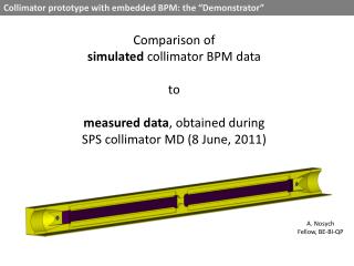
A study comparing simulated collimator BPM data to measured data from the SPS collimator MD in June 2011. The collimator prototype includes advanced features like embedded BPMs and jaw tapering. The experiment involved precise beam positioning and correction of measurement errors. Differences between measurements and simulations were analyzed, and a method for data correction was proposed.

E N D
Collimator prototype with embedded BPM: the “Demonstrator” Comparison of simulatedcollimator BPM data to measured data, obtained during SPS collimator MD (8 June, 2011) A. Nosych Fellow, BE-BI-QP
Model of the Collimator prototype with embedded BPM: the “Demonstrator” EM simulation is done with CST Particle Studio Left jaw with BPMs at the ends, middle buttons are not considered in simulation Graphite R4550 r = 13 mWm Copper r = 17 nWm S-steel 316L Special jaw tapering with extrusions to emulate the RF contacts
1. Start of the experiment in SPS Collimator is parked Beam at arbitrary location* (single coasting bunch) *since the vertical beam location is irrelevant, consider the beam somewhere on X axis Jaw gap (D) = 60.8 mm (parked) Button distance (B) = D + 21 mm Bunch length (4sigma) = 2.1 ns Left jaw downstream view Right jaw beam Collimator center
3. Center jaws around beam, move jaws around beam Experiments are done with gaps of [around] D = 28, 24, 20, 16, 12 and 8 mm. Centering is done via microcontroller. Beam position is measured in several locations: at [around] 0%, 20%, 40%, 60% and 80% of each D/2 (half gap size) Exact jaws positions are recorded in Timber at every step. At 8 mm 20% offset the BLMs detect losses and jaws are not moved any closer. D = 28 mm 0% 20% 40% 60% 80% D = 24 mm 0% 20% 40% 60% D = 20mm 0 20 40 60 80% D =16 0 20 40 60% D =12 0 20 40% D =8 0 20%
5. Raw measurement vs. simulation Examples of raw beam position measurement compared to simulation. 80% 60% 60% 40% 40% 20% beam offset 20% beam offset beam centered beam centered Raw measurement can be corrected for initial jaws offset and for electronic offset.
4. Differences between measurement and simulation setup • Measurement errors NOT under control: • Difficult to align jaws at precise positions, keeping constant gap => different geometric setup at every step => imprecise comparison with simulation; • Problems with data transmission from Microcontroller to logging device => unknown error in measured data; • Beam is never parallel to jaws in reality => upstream/downstream measurements lead to different results and must be treated separately; • Real collimator buttons are retracted for extra 0.5 mm from the tapered collimator surface, which adds 1 mm to total button distance (see pictures on right): 21 mm in reality vs. 20 mm in simulations => plays bigger role as jaws get closer. Real collimator 0.5 mm 10 mm 10 mm Model Measurement errors under control: Jaw offset for centered beam (precisely known); Estimated location of electrical center of the linearity characteristic (approximate).
5. Remove initial jaw offset from raw data Raw data correction, step 1: correcting for beam center Given the collimator natural coordinate system (x’,y’) with off-centered beam, Introduce a new coordinate system (x,y) centered around the beam. D Beam centered y´ y xc xR x´ x Collimator center
6. Remove electronics’ offset from raw data Raw data correction step 2: overlay linearity characteristics to have a common “electrical center”: yerr xc Example: Raw and corrected non-linearity of a 28mm gap
7. Measurement vs. simulation. Gaps of 28, 24 and 20 mm Non-linearity of beam position measurement Jaw dist, D = 28 mm 0% 20% 40% 60% 80% Button dist, B = 48 mm D = 24 mm 0% 20% 40% 60% B = 44 mm D = 20mm 0 20 40 60 80% B = 40 mm
7. Measurement vs. simulation. Gaps of 16, 12 and 8 mm Non-linearity of beam position measurement D = 16 mm 0 20 40 60% B = 36 mm D = 12 mm 0 20 40% B = 32 mm D = 8 mm 0 20% B = 28 mm
8. Measurement vs. simulation: slopes Measurement: Up-stream non-linearity slopes (per point) Measurement: Down-stream non-linearity slopes (per point) Simulation: map of slopes vs. button distances, ranging from parked jaws at 60 mm (B=80mm), to operational distance of 2mm (B=22mm) Bad news: linear non-linear non-linear Good news: Both non-linearities can be predicted trough simulation.
9. Conclusion • Conclusion: • Despite the presence of several error sources and imperfections of measurement, a good agreement between simulation and measurement is observed. • Horizontal correction factor is non-linear with respect to jaw gap. • Behavior of real collimator BPM signals for various jaw gaps can be predicted through simulation. • Correction factors can be derived from simulated signals for several jaw gaps and building a fit to cover the whole jaw motion range. Anticipation: Since several major error sources are already understood/eliminated, more collimator BPM MDs are desired throughout 2012 to improve validation of the model. Several short measurements (with several gaps) would be sufficient. Acknowledgements: Marek Gasior, Christian Boccard.
10. Reserved slide Transverse non-linearity maps
![Data Modeling [Comparison of data modeling techniques ]](https://cdn0.slideserve.com/205866/data-modeling-comparison-of-data-modeling-techniques-dt.jpg)


![Data Modeling [Comparison of data modeling techniques ]](https://cdn3.slideserve.com/6795343/data-modeling-comparison-of-data-modeling-techniques-dt.jpg)