Download
1 / 21
210 likes | 385 Vues
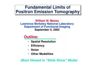
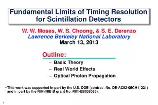
Outline: Basic Theory Real World Effects Optical Photon Propagation. Fundamental Limits of Timing Resolution for Scintillation Detectors. W. W. Moses, W. S. Choong , & S. E. Derenzo Lawrence Berkeley National Laboratory March 13, 2013.

E N D
Outline: Basic Theory Real World Effects Optical Photon Propagation Fundamental Limits of Timing Resolutionfor Scintillation Detectors W. W. Moses, W. S. Choong, & S. E. DerenzoLawrence Berkeley National Laboratory March 13, 2013 • This work was supported in part by the U.S. DOE (contract No. DE-AC02-05CH11231) and in part by the NIH (NIBIB grant No. R01-EB006085). 1
Zoom In… The Fundamentals… I(t) = I0 exp(-t/) Light Output = I0 • Timing Determined by I0(Initial PE Rate) • I0=Eϒ(Light Output / ) Collect_EffQuantum_Eff • Look at Arrivial Times of Individual Photoelectrons 2
Time Jitter of nth Photoelectron PE Rate = 100 PE/ns PE Rate = 1000 PE/ns “Poor” TOFPET “Good” TOFPET • LSO (40ns, 30k ph/MeV) • PMT (25% QE), 50% CE • 50 PE/ns • LaBr3 (15ns, 72k ph/MeV) • UBA PMT (50% QE), 75% CE • 900 PE/ns • Jitter (fwhm) = 2.35 sqrt(n) / I0 • First Photoelectron has Least Jitter 3
Timing Pickoff Trig. Level • Leading Edge Discriminator Often Used • If the trigger level is at n photoelectrons,timing resolution ≈ jitter of nth photoelectron • Valid if PD_Rise ≪ PE Jitter ≪ PPD_Fall(individual photoelectrons resolved) Trig. Level • First PE Traditionally Favored • Described by Post & Schiff in 1960 4
Problem: Predicts Incredible Timing • “Poor” TOFPET • LSO (40ns, 30k ph/MeV) • Standard PMT (25% QE) • 50% CE • 50 PE/ns • “Good” TOFPET • LaBr3 (15ns, 72k ph/MeV) • UBA PMT (50% QE) • 75% CE • 900 PE/ns ⇒ 66 psfwhm PET Timing ⇒ 3.7 psfwhm PET Timing 5
Why? Real World Effects • Overlap of photoelectron pulses • Photodetector transit time jitter(Gaussian) • Photodetector rise & fall time(Bi-Exponential) • Intrinsic scintillator rise time(Exponential) • Optical transport in scintillator(Exponential) Our Contribution • Estimated Through Monte Carlo Simulation • Described by Hyman in 1964 & 1965 6
“Real World” Probability Density Function “Abrupt” Rising Edge Disappears… 7
“Real World” Jitter of nth Photoelectron PE Rate = 100 PE/ns PE Rate = 1000 PE/ns • First PE No Longer Has Lowest Jitter • Broad Minimum – Many PEs Have Similar Jitter 8
Run Lots of Monte Carlo • 820 Combinations • Initial Photoelectron Rate I0: 10 – 10,000 PE/ns • Intrinsic Scintillator Rise Time: 0 – 1 ns (exponential) • Photodetector Transit Time Jitter: 0 – 0.5 ns fwhm (Gauss) • Optical Photon Propagation Time: 0 – 0.2 ns (exponential) • Convolve w/ Photodetector Response to Simulate Analog Out(results insensitive to PD response, including rise time) • Simulate Leading Edge Discriminator withOptimized Threshold for Each Combination • Get Tables of Simulated Timing Resolution • Fit Tables to Analytic Formula 9
Analytic Formula for Timing Resolution Timing Resolution (ns fwhm) = B / sqrt(I0) B (r, d, J,I0) = sqrt[ 5.545 I0-1 + 2.424 ( r+ d ) + 2.291 J + 4.938 rd + 3.332 J2+ 8.969 J2 I0-1/2 + 9.821( r2+ d2 ) I0-1/2 − 0.6637( r+ d ) I0-1/2− 3.305 J ( r+ d ) − 6.149 JI0-1/2 − 0.3232 ( r2+ d2 ) − 3.530 J3− 5.361 J rd − 9.287 rdI0-1/2 − 5.814 J𝜏( r3+ d3 ) ] I0 =Eϒ(Light Output / ) Collect_EffQuantum_Eff(photons/MeV/ns) r = Intrinsic Scintillator Rise Time (ns) J = Photodetector Transit Time Jitter (ns) d = Optical Photon Propagation “Decay Time” (ns) Formula Obtained Using “Eureqa” Software 10
Fit vs. True Value for B • Excellent Fit (RMS Deviation ~ 2%) • For Virtually All Conditions, 0.5 < B < 2 11
Other Observations • No Other Significant Dependencies • Photodetector Rise Time • Photodetector Fall Time • Timing Resolution Using “Optimal” Estimator that Uses All Detected Photoelectrons is ≤15% Better than Leading Edge Timing(for r= 0.5 ns, d = 0.1 ns, J = 0.2 ns) • Paper submitted to Phys. Med. Biol. 12
Timing Resolution Predicted If You Know: ✔ • Initial Photoelectron Rate I0 • Gamma Ray Energy • Scintillator Luminosity • Scintillator Decay Time • Collection Efficiency • Quantum Efficiency • Intrinsic Scintillator Rise Time • Photodetector Transit Time Jitter • Optical Photon Propagation Time ✔ ✔ ✔ ✔ ✔ ✔ ✔ What Value to Use for Propagation Time??? 13
Estimate Using GEANT / GATE / DETECT • Index of Refraction n= 1.82 (same as LSO) • Light Generated as a Delta Function in Timeat Random Positions in the Scintillator • Three Surface Finishes Simulated • Polished • Chemically Etched • Rough • Two Simulation Types for Each Surface • “Unified Model” (σα = 0°, 6°, and 12°) • “RealReflector” (measured values in LUT) 14
Basic Pulse Shape Photo-detector Reflector 3x3x30 mm Amplitude Polished Surfaces Delay “Decay” Time Well-Described By Exponential Decay 15
Simplifying the Simulation L Photo-detector Reflector x ∞ 3 x 3 x ∞ mm Photo-detector 2L – x • Run Single Simulation w/ Infinitely Long Crystal • Superpose Signals from Positions x and 2L–x • Reflected Signal Less Important for Timing… 16
Simulation Results (Polished & Etched) Delay = Distance * nc 17
Simulation Results (Rough) • Unified “Rough” Very Similar to “Etched” and “Polished” • Lookup “Rough” is VERY Different 18
Simulation Results (Rough Surface) Lookup Table Unified Model Different Models Predict Very Different Behavior 19
Scaling Crystal Dimensions L W t Photo-detector x 1.5 L 1.5 t Photo-detector 1.5 W 1.5 x • Simulations Run on 3 mm x 3 mm Crystal • Results for a W x W Crystal Can Be Found ByMultiplying All Distances & Times on Graphs by W/3 20
Conclusions • Simulation used to estimate timing resolution for many combinations of scintillation detector parameters • Includes virtually all known effects • Results encapsulated in “simple” formula that predicts timing resolution • All inputs to formula readily obtained(including optical dispersion in crystal) • Needs experimental validation! 21