Download
1 / 41
410 likes | 529 Vues
This work explores cutting-edge techniques for analyzing high-energy physics (HEP) collider data using two primary frameworks: Quaero for hypothesis testing and Sleuth for identifying potential new physics phenomena. With the backdrop of the Standard Model, we demonstrate a systematic search across event data, detailing the process from data partitioning and variable selection to likelihood calculations. By reducing analysis time and human bias by significant factors, we aim to reveal any excess events that could indicate novel discoveries, enhancing the robustness and efficiency of research in particle physics.

E N D
Systematic Analysis of HEP Collider Data Sleuth Quaero Optimal binning Bruce Knuteson MIT
“Objects” seen in the detector e b j (the colors are meaningless)
A cartoon collision (An “event”) • 4 objects per event • 3 numbers per object • energy E • directions , • Each event is described by 4object types and 12 numbers 10-16 m
Standard Model the null hypothesis
The theoretical landscape Murayama, Lepton Photon 2003 summary talk
The theoretical landfill www.southampton.gov.uk/government/ environment/waste.htm
Sleuth A detective. (From sleuthhound – a dog, such as a bloodhound, used for tracking or pursuing.)
e Partition the data e+ p b e- p j e+jjbb e+e- e+bb e+3j e+e-2jj e+jj e+μ+ e+ e+ e+e+e- +3jj e+μ-jj ee4j +bb Sleuth
Define variables e+ e- proton anti-proton If new TeV-scale physics enters here outgoing particles will be energetic relative to Standard Model and instrumental backgrounds Use object pT's Sleuth
Search for regions of excess (more data events than expected from background) within that variable space For each final state . . . Input:1 data file, estimated backgrounds • transform variables into the unit box • define regions about sets of data points • Voronoi diagrams • define the “interestingness” of an arbitrary region • the probability that the background within that region fluctuates up to or beyond the observed number of events • search the data to find the most interesting region,R • determineP, the fraction ofhypothetical similar experimentsin which you would see something more interesting thanR • Take account of the fact that we have looked in many different places Output:R,P Sleuth
Run I data Sleuth Results agree with SM expectation Phys.Rev.D62:092004,2000; hep-ex/0006011 Phys.Rev.D64:012004,2001; hep-ex/0011067 Phys.Rev.Lett.86:3712,2001; hep-ex/0011071
# events model-independent general search in same spirit presented by H1 at EPS 2003 watch this space in HERA II
7) Does Sleuth find anything interesting in Run I data? Question: Is it possible to perform a data-driven search for new phenomena? No.A systematic search of many final states reveals no evidence of new high pT physics. 8) Apply to Run II 1) Define final states 6) Can Sleuth find something interesting? Sleuth (yes!) top bkg 2) Define variables p p 3) Define regions 4) Define "interestingness" 5) Run hypothetical similar experiments
Quaero Automating tests of specific hypotheses against HEP collider data NASA astronomy picture of the day Oct 1, 2002 Surface of Mars
Wish list • Reduce analysis time by factor of 10000 • Reduce human bias • Publish data in full dimensionality • Expunge exclusion contours from conference talks • Automate optimization of analyses • Rigorously propagate systematic errors • Increase robustness of results • Easily combine results among different experiments • All of this on the web
Search for New Physics Using Quaero: A General Interface to DØ Event Data Run I data since June 2001 http://quaero.fnal.gov/ hep-ex/0106039 PRL 87 231801
Quaero algorithm overview (you wish to test a hypothesisH) • H events are run through the detector simulation • H, SM, data are partitioned into final states • Variables are chosen automatically • Binning is chosen automatically • A binned likelihood is calculated • Results from different final states are combined • Results from different experiments are combined • Systematic errors are integrated numerically • Result returned
Typical problem true distributions our knowledge wish to determine
Want to provide the strongest evidence possible in favor ofhifhis correct . . . . . . and the strongest evidence possible in favor ofbifbis correct
Figure of MeritM (Choice of binning for likelihood ratio calculation) sum over all possible outcomes of the experiment. # of data eventsdkin each binkis [0,) the evidence obtained in favor ofhin this outcome . . . plus the same thing, but switchhandb minus a penalty term weight outcome by the probability of its occurrence, assuming the validity ofh + ditto forb expected evidence in favor ofhifhis correct
Example #1 Expected # of events / unit of x Expected evidence
Example #2 Expected # of events / unit of x Expected evidence
Multivariate generalization Using the same procedure, create a d-dimensional grid: x e.g., y - or - Use Kernel Density Estimation to reduce the problem to 1-d
FewKDE Typical kernel solution 1) place “bumps of probability” around each Monte Carlo point 2) sum these bumps into a continuous distribution Time cost is O(N2) FewKDE • fit for parameters of five Gaussians • appropriately handle hard physical boundaries
Example #3 h b true distributions (contours) Monte Carlo events f e d c b a e f d c b KDE discriminant
Summary Sleuth model-independent search for new high pT physics Quaero automates tests of specific models Optimal Binningchoosing the bins for binned likelihood ratios Special thanks to: and many others
How “sensitive” is Sleuth to WW eET ? Observed at 2.3 CDF, “Observation of W+W- production . . . .” PRL 78 4536 (1997) 5 events observed on a bkg of 1.20.3 Sleuth
How “sensitive” is Sleuth to tt eETjj ? Observed at 2.1 DØ, “Measurement of the Top Quark Pair Production Cross Section in ppbar Collisions” PRL 79 1203 (1997) 5 events observed on a bkg of 1.40.4 Sleuth
Run I data: eμETX Backgrounds include 1) 2) 3) • fakes • Z • WW • tt • fakes • Z • WW • tt • fakes • Z • WW • tt DØ data DØ data DØ data Excesses corresponding (presumably) to WW and tt Excesses corresponding (presumably) to tt No evidence for new physics Sleuth
An hour’s worth of a typical conference (HCP 2002, Th Oct 10 4-5pm) basically useless
How to choose a set of cuts without bias? signal region data background region
Variables Dimensional Rule of Thumb: > 10d events are needed to adequately populate a d-dimensional space Corollary: analysis should be performed in a space of dimensionality d = log10NMC Prescription: 1.Generate a long (but finite) list of relevant variables TeV:pT, , , ij, Rij, mij, mijk, mijkl LEP:E, , , ij, Rij, mij, mijk, mijkl 2.Order according to decreasing discrepancy (HvsSM) 3.Use the firstdvariables in the list, removing highly correlated variables
Simplification and sample special cases Simplification and special cases Large statistics (NMC, hk) Signal + background s x b bins 1 2 Recover the familiar
Penalty term Origin: wantM =0whenh = b factorizes: MC event weights # MC events # bins can be derived analytically in the case of equal weights is determined empirically (expression holds over five orders of magnitude from 101 < nMC < 106) is simply proportional to the number of bins