Folds
Folds. Field and Lab Measurements. Data Acquired for Folds. Detailed structural analysis requires sampling of: Bedding in sedimentary rock Compositional layering in gneiss Planar fabric (cleavage) with lineation on them Fold elements (attitude of axial plane and hingeline) Shear zones

Folds
E N D
Presentation Transcript
Folds Field and Lab Measurements
Data Acquired for Folds • Detailed structural analysis requires sampling of: • Bedding in sedimentary rock • Compositional layering in gneiss • Planar fabric (cleavage) with lineation on them • Fold elements (attitude of axial plane and hingeline) • Shear zones • Faults, slickensides • Joints
Measuring a fold requires exposing the folded layer with chisel and hammer
Collecting Data • Measure as many folds and their elements as possible • A higher number of folds measured will improve the accuracy of later structural analysis • Measure all structural fabrics in the same folded rock • e.g., cleavage, lineation • relationship to the folds • Plot all the fabric data on the stereonet, and conduct a careful study of the orientation data
Measuring a Fold • Folds are completely defined by the attitude of their: • Axial plane (strike, dip) • Hingeline or axis (trend, plunge) • Most folds are non-cylindrical • Break such folds into smaller segments (domains) where they have a homogeneous fabric (i.e., are cylindrical), then measure them • Then measure the attitude of several tangent planes on the two limbs
Measure the attitude of at least two folded layers (e.g., bedding (b or S0), cleavage (c or S1) on both limbs (note them down as: b1, b2, b3, b4 in your notebook) • Measure the attitude of the hingeline (HL), by measuring a pencil parallel to the line connecting points of max. curvature (Note: measure the trend down-plunge!) • If HL cannot be measured, measure as many axial traces (AT) as possible; then line them up on a same great circle • Measure the axial plane (AP) directly, if possible • AP contains the HL (a pencil) and the axial trace (AT) (a second pencil) on the profile plane (plane perpendicular to the hingeline) or any other plane
Plot the Fold Data(-diagram) • Plot the fold elements using an equal-area stereonet • Plot the normal or pole to each folded layer as a point, with a consistent symbol, e.g., use: or for the pole to folded bedding or cleavage • Plot the normal to the axial plane (symbol: ) • The best-fit great circle through the poles defines the profile plane (plane normal to the axis) • The pole to the profile plane is the fold axis (symbol:) • Plot the hingeline () and compare it with the axis () • Check to see if the and/or lie on the axial plane if it is measured in the field or determined indirectly
Determine the axis at the pole of the profile plane profile plane
Cylindrical Folds(-diagram) • Plot the folded layers as cyclographic projections (i.e., great circles) • Determine the fold () axis at the intersection of all the cyclographs (they do not intersect exactly at a point!) • The axis and the axis are generally the same • The diagram is more cluttered than the diagram • We commonly use both of these diagrams in our fold analysis
Davis and Reynolds, 1997Determine the axis by intersecting the clyclographs of the folded layers
The Interlimb Angle • The poles to the two limbs of a fold may not spread over the 180o sector of the profile plane (i.e., does not define a full great circle) • In this case, the interlimb angle is the angle between the two dominant clusters (maxima) of the poles (of the two limbs) measured on the profile plane • If the fold has straight limbs (e.g. chevron fold), the poles to the two limbs define two maxima • In such a case, the fold axis is the intersection of the two planes (great circles) drawn perpendicular to these two maxima
Construction of the Axial Plane • The axial plane is the great circle that includes the axis (hingeline) and any of the measured axial traces (in the field or on map, anywhere on the fold) • The axial plane is the great circle that contains at least two axial traces on two random sections along the axial plane (none has to be the hingeline) • In a symmetric fold, the axial plane may be assumed to be the bisector of the fold containing the fold axis • Folds may have a foliation parallel to or fanning about the axial plane of the fold
Construction of the Fold Axis from Intersections • The fold axis can also be determined from: • (So x S1) i.e., intersection of the hinge plane or axial plane (e.g. S1) and folded surface (So), where So is the original surface such as bedding or banding in a lava flow, and S1 is the first generation surface such as the axial plane of first generation fold or an axial-plane cleavage. • The (So x S1) intersection of an axial-plane foliation, S1 and folded layer, So • The (So x So) intersection of several tangent planes to the folded layer in the hinge area of the fold ( axis)
Fold axis = So x S1 S1 So
Fold axis = So x S1Pole to the fanning S1 lie on the profile plane S1 S1 S1 S1 S1 S1 So
Fold Classification – Ramsay 1967 • Start with a profile plane view of a fold (constructed by rotation, or photographed in the field looking downplunge). • Mark the hinge points and inflection points on the two bounding surfaces of the folded layer • Draw the tangents to the folded layer at the hinge points. This is the zero dip ( = 0) reference • At = 0, measure the orthogonal hinge thickness to • Construct other tangents at other angles • Measure the orthogonal thickness (t) between these tangents for these angles • Determine the ratio: t’ = t /to • Plot t’ as ordinate against as abscissa • Repeat for all values of
Fold Classification - Parallel Folds • Normal thickness (t), perpendicular to the layer, is constant throughout the fold, i.e., t’ = t /to = 1 • Some parallel fold are concentric; i.e., have constant, circular curvature • Parallel folds are typical of competent layers • Layer thickness, measured parallel to the axial plane, is greater on the limbs (T) than that around the hinge (To), i.e., (T> To)
Similar Folds • Have variation in their layer thickness, t • The orthogonal layer thickness reduces on the limb • The orthogonal thickness varies as: t’ = cos • The curvature of the bounding surfaces are identical (hence the word ‘similar’) • The layer thickness measured parallel to the axial plane (T) is constant (T = To = to)
Similar fold T = To = to
Intermediate Fold Styles – Ramsay 1967 • The similar and parallel folds are not the end members of fold style. Other styles fall outside of these two • Progressive deformation (e.g., flattening) may change one geometry to another • Ramsay proposed analyzing the variation of the t layer thickness with the angle of dip within a quarter fold wave sector
Dip Isogons • Lines joining points of equal dip (normal to tangents) • Drawn at different angles (at 10o intervals) • Isogons can be parallel, converging, or diverging • The sense is from the outer arc to the inner arc • Parallel isogons: • The average inner and outer curvatures are equal • Converging isogons: • Inner arc curvature exceeds that of outer arc • Divergent isogons: • Outer arc curvature exceeds that of the inner arc.
Fold Classification … • On the t‘ against diagram: • All other folds fall on either side of the two lines: t‘ = 1 (parallel fold = class 1B) t‘ = cos (similar fold = class 2) • Class 1A folds lie above class 1B parallel folds. • Class 1A folds are thicker on the limb than near the hinge • Class 1C, class 2, and class 3 folds all show thinning on the limb