Understanding Spatial Modeling in Raster Format: Key Concepts and Practical Challenges
This lecture outlines the fundamentals of spatial modeling in raster format, focusing on key concepts such as raster cells, resolution, and attribute data linking. It discusses the implications of cell size, including the trade-off between spatial precision and data file size. The lecture also addresses issues with determining cell values and procedures for filtering raster data. Techniques for georeferencing and mosaicking raster images are examined, with emphasis on color adjustment and spatial registration. Lastly, the importance of raster data in creating effective base maps is highlighted.

Understanding Spatial Modeling in Raster Format: Key Concepts and Practical Challenges
E N D
Presentation Transcript
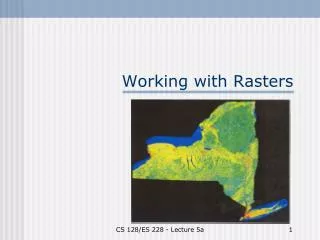
Working with Rasters CS 128/ES 228 - Lecture 5a
Spatial modeling in raster format • Basic entity is the cell • Region represented by a tiling of cells • Cell size = resolution • Attribute data linked to individual cells CS 128/ES 228 - Lecture 5a
Issue #1 - resolution Larger cells: • less precise spatial fix • line + boundary thickening • features too close overlap - less detail possible Fig. 3.10, 3rd ed. CS 128/ES 228 - Lecture 5a
Why not always use tiny cells? • Data inputs may have limited spatial resolution - pixel size for aerial, satellite photos- reliability of coordinate measurements • Size of data files • Speed of analysis CS 128/ES 228 - Lecture 5a
Issue #2 - determining cell values • Data inputs may already contain cell values: aerial, satellite photos • Cell values may be assigned: “pseudocolors” • Ultimately all cell values must be coded numerically CS 128/ES 228 - Lecture 5a
Image depth • minimum = 1 bitB/W image or P/A data • 8-bit image = 256 levels of gray (can be pseudo-colored) • 24-bit image = true-color. Each primary color has separate layer CS 128/ES 228 - Lecture 5a
Determining cell values CS 128/ES 228 - Lecture 5a
Filtering raster data • Neighborhood averaging • Smoothes “holes” and transitions • Other techniques available Chang 2002, p. 203 CS 128/ES 228 - Lecture 5a
Issue #3 - layers in raster format • Each layer must be referenced in common coordinates • Thematic data can be combined and revised (reclassified) CS 128/ES 228 - Lecture 5a
Analysis by raster overlay Fig. 6.17, 3rd ed. CS 128/ES 228 - Lecture 5a
Lack of spatial registration CS 128/ES 228 - Lecture 5a
Georeferencing raster images • Spatial coordinates may be absent or purely map coordinates (i.e. inches from one corner) • Control points: point features visible on both the image and the map • Linear or nonlinear transformations • “Rubber sheeting” CS 128/ES 228 - Lecture 5a
Issue #4 – mosaicking rasters http://www.microimages.com/featupd/v57/mosaic/ CS 128/ES 228 - Lecture 5a
Mosaicking: mismatched tiles Ex. Aerial photographs of Kinzua Reservoir What do you suppose caused the drastic differences in water clarity in the lake? Google map of Onoville, NY. Accessed 6 Oct 2008 CS 128/ES 228 - Lecture 5a
Mosaicking: adjusting color values Histogram matching: • Computer compiles histogram of color (or gray) values in 1 tile • 2nd tile’s colors adjusted to match CS 128/ES 228 - Lecture 5a
Raster data editing CS 128/ES 228 - Lecture 5a
Clip to rectangle ... CS 128/ES 228 - Lecture 5a
… vs.clip to shapefile CS 128/ES 228 - Lecture 5a
Summary • A huge amount of spatial data are available in raster format • Rasters make excellent “base maps” • Easy to layer but watch coordinate systems! • Difficult/impossible to edit or reproject USGS Digital Raster Graphic (DRG) Quadrangle(1:24,000 scale - UTM Zone 17, NAD 27) CS 128/ES 228 - Lecture 5a