Download
1 / 62
650 likes | 944 Vues
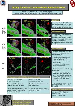
Quality Control of Weather Radar Data. Valliappa.Lakshmanan@noaa.gov National Severe Storms Laboratory & University of Oklahoma Norman OK, USA http://cimms.ou.edu/~lakshman/. Weather Radar. Weather forecasting relies on observations using remote sensors.

E N D
Quality Control of Weather Radar Data Valliappa.Lakshmanan@noaa.gov National Severe Storms Laboratory & University of Oklahoma Norman OK, USA http://cimms.ou.edu/~lakshman/ Valliappa.Lakshmanan@noaa.gov
Weather Radar • Weather forecasting relies on observations using remote sensors. • Models initialized using observations • Severe weather warnings rely on real-time observations. • Weather radars provide the highest resolution • In time: a complete 3D scan every 5-15 minutes • In space: 0.5-1 degree x 0.25-1km tilts • Vertically: 0.5 to 2 degrees elevation angles Valliappa.Lakshmanan@noaa.gov
NEXRAD – WSR-88D • Weather radars in the United States • Are 10cm Doppler radars • Measure both reflectivity and velocity. • Spectrum width information also provided. • Very little attenuation with range • Can “see” through thunderstorms • Horizontal resolution • 0.95 degrees (365 radials) • 1km for reflectivity, 0.25km for velocity • Horizontal range • 460km surveillance (reflectivity-only) scan • 230km scans at higher tilts, and velocity at lowest tilt. Valliappa.Lakshmanan@noaa.gov
NEXRAD volume coverage pattern • The radar sweeps a tilt. • Then moves up and sweeps another tilt. • Typically collects all the moments at once • Except at lowest scan • The 3dB beam width is about 1-degree. Valliappa.Lakshmanan@noaa.gov
Beam path • Path of the radar beam • slightly refracted • earth curvature • Standard atmosphere: 4/3 • Anamalous propagation • Beam heavily refracted • Non-standard atmospheric condition • Ground clutter: senses ground. Valliappa.Lakshmanan@noaa.gov
Anomalous Propagation • Buildings near the radar. • Reflectivity values correspond to values typical of hail. • Automated algorithms severely affected. Valliappa.Lakshmanan@noaa.gov
AP + biological • North of the radar is some ground-clutter. • The light green echo probably corresponds to migrating birds. • The sky is actually clear. Valliappa.Lakshmanan@noaa.gov
AP + precipitation • AP north of the radar • A line of thunderstorms to the east of the radar. • Some clear-air return around the radar. Valliappa.Lakshmanan@noaa.gov
Small cells embedded in rain • The strong echoes here are really precipitation. • Notice the smooth green area. Valliappa.Lakshmanan@noaa.gov
Not rain • This green area is not rain, however. • Probably biological. Valliappa.Lakshmanan@noaa.gov
Clear-air return • Clear-air return near the radar • Mostly insects and debris after the thunderstorm passed through. Valliappa.Lakshmanan@noaa.gov
Chaff • The high reflectivity lines are not storms. • Metallic strips released by the military. Valliappa.Lakshmanan@noaa.gov
Terrain • The high-reflectivity region is actually due to ice on the mountains. • The beam has been refracted downward. Valliappa.Lakshmanan@noaa.gov
Radar Data Quality • Radar data is high resolution, and is very useful. • However, it is subject to many contaminants. • Human users can usually tell good data from bad. • Automated algorithms find it difficult to do so. Valliappa.Lakshmanan@noaa.gov
Motivation • Why improve radar data quality? • McGrath et al (2002) showed that the mesocyclone detection algorithm (Stumpf et al, Weather and Forecasting, 1999) produces the majority of its false detections in clear-air. • The presence of AP degrades the performance of a storm identification and motion estimation algorithm (Lakshmanan et al, J. Atmos. Research, 2003) Valliappa.Lakshmanan@noaa.gov
Quality Control of Radar Data • An extensively studied problem. • Simplistic approaches: • Threshold the data (low=bad) • High=bad for AP, terrain, chaff • Low=good in mesocylones, hurricane eye, etc. • Vertical tilt tests • Works for AP • Fails farther from the radar, shallow precipitation. Valliappa.Lakshmanan@noaa.gov
Image processing techniques • Typically based on median filtering reflectivity data • Removes clear-air return, but fails for AP. • Fails in spatially smooth clear-air return. • Smoothes the data • Insufficiently tested techniques • Fractal techniques. • Neural network approaches. Valliappa.Lakshmanan@noaa.gov
Steiner and Smith • Journal of Applied Meteorology, 2002 • A simple rule-base. • Introduced more sophisticated measures • Echo top: the highest tilt that has at least 5dBZ. • Works mostly. Fails in heavy AP, shallow precipitation. • Inflections • Measure of variability within a local neighborhood of pixel. • A texture measure suited to scalar data. • Their hard thresholds are not reliable. Valliappa.Lakshmanan@noaa.gov
Radar Echo Classifier • Operationally implemented on US radar product generators • Fuzzy logic technique (Kessinger, AMS 2002) • Uses all three moments of radar data • Insight: targets that are not moving have zero velocity, and low spectrum width. • High reflectivity values usually good. • Those that are not moving are probably AP. • Also makes use of Steiner-Smith measures • Not vertical (echo-top) features (to retain tilt-by-tilt ability) • Good for human users, but not for automated use Valliappa.Lakshmanan@noaa.gov
Finds the good data and the AP. But can not be used to reliably discriminate the two on a pixel-by-pixel basis. Radar Echo Classifier Valliappa.Lakshmanan@noaa.gov
Quality Control Neural Network • Compute texture features on three moments. • Vertical features on latest (“virtual”) volume • Can clean up tilts as they arrive and still utilize vertical features. • Train neural network off-line on these features • to classify pixels into precip or non-precip at every scan of the radar. • Use classification results to clean up the data field in real-time. Valliappa.Lakshmanan@noaa.gov
The set of input features • Computed in 5x5 polar neighborhood around each pixel. • For velocity and spectrum width: • Mean • Variance (Kessinger) • value-mean Valliappa.Lakshmanan@noaa.gov
Reflectivity Features • Lowest two tilts of reflectivity: • Mean • Variance • Value-mean • Square diff of pixel values (Kessinger) • Homogeneity • radial inflections (Steiner-Smith) • echo size • found through region-growing Valliappa.Lakshmanan@noaa.gov
Vertical Features • Vertical profile of reflectivity • maximum value across tilts • weighted average with the tilt angle as the weight • difference between data values at the two lowest scans (Fulton) • echo top height at a 5dBZ threshold (Steiner-Smith) • Compute these on a “virtual volume” Valliappa.Lakshmanan@noaa.gov
Training the Network • How many patterns? • Cornelius et al. (1995) used a neural network to do radar quality control • Resulting classifier not useful • discarded in favor of fuzzy logic Radar Echo Classifier. • Used < 500 user-selected pixels to train the network. • Does not capture the diversity of the data. • Skewed distribution. Valliappa.Lakshmanan@noaa.gov
Diversity of data? • Need to have data cases that cover • Shallow precipitation • Ice in the atmosphere • AP, ground-clutter (high data values that are bad) • Clear-air return • Mesocyclones (low data values that are good) Valliappa.Lakshmanan@noaa.gov
Distribution of data • Not a climatalogical distribution • Most days, there is no weather, so low reflectivities (non-precipitating) predominate. • We need good performance in weather situations. • Need to avoid bias in selecting pixels – choose all pixels in storm echo, for example, not just the storm core • Neural networks perform best when trained with equally likely classes • At any value of reflectivity, both classes should be equally likely • Need to find data cases to meet this criterion. • Another reason why previous neural network attempts failed. Valliappa.Lakshmanan@noaa.gov
Distribution of training data by reflectivity values Valliappa.Lakshmanan@noaa.gov
Training the network • Human experts classified the training data by marking bad echoes. • Had access to time-sequence and knowledge of the event. • Training data was 8 different volume scans that captured the diversity of the data. • 1 million patterns. Valliappa.Lakshmanan@noaa.gov
The Neural Network • Fully feed-forward neural network. • Trained using resilient propagation with weight decay. • Error measure was modified cross-entropy. • Modified to weight different patterns differently. • Separate validation set of 3 volume scans used to choose the number of hidden nodes and to stop the training. Valliappa.Lakshmanan@noaa.gov
Emphasis • Weight the patterns differently because: • Not all patterns are equally useful. • Given a choice, we’d like to make our mistakes on low reflectivities. • We don’t have enough “contrary” examples. • Texture features are inconsistent near boundaries of storms. • Vertical features unusable at far ranges. • Does not change the overall distribution to a large extent. Valliappa.Lakshmanan@noaa.gov
Histograms of different features • The best discriminants: • Homogeneity • Height of maximum • Inflections • Variance of spectrum width. Valliappa.Lakshmanan@noaa.gov
Generalization • No way to guarantee generalization • Some ways we avoided overfitting • Use the validation set (not the training set) to decide: • Number of hidden nodes • When to stop the network training • Weight-decay • Limited network complexity • <10 hidden nodes, ~25 inputs, >500,000 patterns • Emphasize certain patterns Valliappa.Lakshmanan@noaa.gov
Untrainable data case • None of the features we have can discriminate the clear-air return from good precipitation. • Essentially removed the migratory birds from the training set. Valliappa.Lakshmanan@noaa.gov
Velocity • We don’t always have velocity data. • In the US weather radars, • Reflectivity data available to 460km • Velocity data available to 230km • But higher resolution. • Velocity data can be range-folded • Function of Nyquist frequency • Two different networks • One with velocity (and spectrum width) data • Other without velocity (or spectrum width) data Valliappa.Lakshmanan@noaa.gov
Choosing the network • Training the with-velocity and without-velocity networks • Shown is the validation error as training progresses for different numbers of hidden nodes • Choose 5 nodes for with-velocity (210th epoch) and 4 nodes for without-velocity (310th epoch) networks. Valliappa.Lakshmanan@noaa.gov
Behavior of training error • Training error keeps decreasing. • Validation error starts to increase after a while. • Assume that point this happens is where the network starts to get overfit. Valliappa.Lakshmanan@noaa.gov
Performance measure • Use a testing data set which is completely independent of the training and validation data sets. • Compared against classification by human experts. Valliappa.Lakshmanan@noaa.gov
Receiver Operating Characteristic • A perfect classifier would be flush top and flush left. • If you need to retain 90% of good data, then you’ll have to live with 20% of the bad data when using the QCNN • Existing NWS technique forces you to live with 55% of the bad data. Valliappa.Lakshmanan@noaa.gov
Performance (AP test case) Valliappa.Lakshmanan@noaa.gov
Performance (strong convection) Valliappa.Lakshmanan@noaa.gov
Test case (ground clutter) Valliappa.Lakshmanan@noaa.gov
Test case (small cells) Valliappa.Lakshmanan@noaa.gov
Summary • A radar-only quality control algorithm • Uses texture features derived from 3 radar moments • Removes bad data pixels corresponding to AP, ground clutter, clear-air impulse returns • Does not reliably remove biological targets such as migrating birds. • Works in all sorts of precipitation regimes • Does not remove bad data except toward the edges of storms. Valliappa.Lakshmanan@noaa.gov
Multi-sensor Aspect • There are other sensors observing the same weather phenomena. • If there are no clouds on satellite, then it is likely that there is no precipitation either. • Can’t use the visible channel of satellite at night. Valliappa.Lakshmanan@noaa.gov
Surface Temperature • Use infrared channel of weather satellite images. • Radiance to temperature relationship exists. • If the ground is being sensed, the temperature will be ground temperature. • If satellite “cloud-top” temperature is less than the surface temperature, cloud-cover exists. Valliappa.Lakshmanan@noaa.gov
Spatial and Temporal considerations • Spatial and temporal resolution • Radar tilts arrive every 20-30s • High spatial resolution (1km x 1-degree) • Satellite data every 30min • 4km resolution • Surface temperature 2 hours old • 20km resolution • Fast-moving storms and small cells can pose problems. Valliappa.Lakshmanan@noaa.gov
Spatial … • For reasonably-sized complexes, both satellite infrared temperature and surface temperature are smooth fields. • Bilinear interpolation is effective. Valliappa.Lakshmanan@noaa.gov
Temporal • Estimate motion • Use high-resolution radar to estimate motion. • Advect the cloud-top temperature • Based on movement from radar • Advection has high skill under 30min. • Assume surface temperature does not change • 1-2 hr model forecast has no skill above persistence forecast. Valliappa.Lakshmanan@noaa.gov
Cloud-cover: Step 1 • Satellite infrared temperature field. • Blue is colder • Typically higher storms • A thin line of fast-moving storms • A large thunderstorm complex Valliappa.Lakshmanan@noaa.gov