Download

1 / 20
200 likes | 351 Vues
RFI mitigation for the Parkes Galactic All Sky Survey (GASS). Peter M.W. Kalberla Argelander-Institut für Astronomie Bonn. Galactic All Sky Survey (GASS). N. M. McClure-Griffiths, D. J. Pisano, M. R. Calabretta, H. Alyson Ford, Felix J. Lockman, L. Staveley-Smith,

E N D
RFI mitigation for the Parkes Galactic All Sky Survey (GASS) Peter M.W. Kalberla Argelander-Institut für Astronomie Bonn
Galactic All Sky Survey (GASS) N. M. McClure-Griffiths, D. J. Pisano, M. R. Calabretta, H. Alyson Ford, Felix J. Lockman, L. Staveley-Smith, P. M. W. Kalberla, J. Bailin, L. Dedes, S. Janowiecki, B. K. Gibson, T. Murphy, H. Nakanishi, K. Newton-McGee, J. Kerp, B. Winkel McClure-Griffiths et al. (2009) Kalberla et al. (2010)
GASS: survey parameters • 13 beam receiver • 21-cm line survey of the Galactic HI emission • Declinations δ < 1 deg • (-500) < -468 < vLSR < +468 < (+500) km/s • Δv = 1 km/s • In-band frequency switching, Δv = 660 km/s • Beam FWHM 14.4 arcmin • OTF mapping in RA and DEC, two coverages • 2.8·107 spectra, 5 sec dumps, noise ~0.4 K • 10 observing sessions between 2005 and 2006 • FITS maps: noise at full resolution (15.6 arcmin): 60 mK
Problems • RFI at fixed frequency without significant variation in time • Causing in many cases negative signals (ghosts) • Broad lines (Δv ~ 15 km/s) in March 2006 • Bandpass ghosts from HVC gas due to folding • Footprints: strong RFI signals for short time intervals • Ringing (Gibbs phenomenon) from correlator
First step: Use livedata flags • LAB data are used for fitting the instrumental baseline • At that stage it is easy to replace channels flagged by livedata during first stage of reduction with LAB data • Alternatively flagged data can be interpolated from neighboring channels of Parkes data • The replacement using LAB is far better!! • 0.1% of all data affected
Median filter (at any observed position) • Determinemedian, mean and rms fluctuations within a radius of 6 arcmin (consistent with HIPASS) • Find channels that have • High rms scatter (> 3 σrms)and • Large differences between median and mean (>σm) • Replace data that deviate > 2 σm from median by median • Do not filter for T > 0.5 K (T > 2 K at b > 10 deg) • Do not filter at positions with continuum > 200 mJy • 0.07% of all data affected
Peirce criterion (1852) AJ 2, 161 • Criterion for the rejection of doubtful observations • Cutoff limit for exclusion of outliers depends on number of available data points • For 40 profiles (typically) a 2 σrms limit is adequate if about 10% of the data are suspect • A 1.6 σrms limit would be adequate if about 20% of the data are suspect • We use a fixed 2 σrms limit with deviations from the median
Extra treatment: • Eliminate spectra with high noise (>3 times average) and with more than 30 flagged channels (0.3% affected) • Bandpass ghosts can be minimized by median filtering • RFI in March 2006 (broad Gaussian lines) • Fit parameters • Flag data accordingly • Median filtering as usual RFI • Emission lines > 2 K • No automatic filtering • Inspect data and filter only those regions that are affected
Reorganize database for computational reasons • 300 GBsdfits files with 2.8·107 spectra are hard to handle • Generate compressed random access database • 135 GB in single file, pointer information • fast access of individual profiles • Benefit of new data format: • Allows fast filtering • Very fast on-the-fly processing of FITS cubes
21cm line work and Darwinism • Correction for stray radiation suffers from detailed observations of the antenna diagram • Antenna parameters: • Model parameters need to be self-consistent • ~60 different runs • Baseline correction: • Code and parameters need to survive • ~50 different versions necessary • RFI mitigation • Comparison of all profiles at any position within 6 arcmin (109 cases) • >2 CPU years in total Does the solution survive? How are the Profiles today? ? Hornet magazine, 1871
Summary • RFI post-processing needs redundancy • Typically no more that 25% of the data are bad • Limit: 50% • Fast data access necessary for filtering • New data format needed (random access) • Advantages: generation of FITS cubes very fast • Replace bad data by LAB data or by median • Surprisingly simple recipe to use other data
This all was about… RFI in the protected band But <0.5% of data affected