High-order codes for astrophysical turbulence
540 likes | 678 Vues
This document covers high-order numerical codes tailored for astrophysical turbulence, highlighting the Pencil Code's features and capabilities. Key topics include Kolmogorov spectrum behaviors, nonlinearity, and power law implications in cosmic structures. The study investigates direct simulations at resolutions like 10243 and discusses challenges such as hyperviscosity, normal diffusivity, and the bottleneck effect in turbulence. Additionally, it delves into the efficiency of high-order schemes, parallelization, and various modules for different astrophysical applications. This work is relevant for researchers focused on turbulent flow dynamics in astrophysical contexts.

High-order codes for astrophysical turbulence
E N D
Presentation Transcript
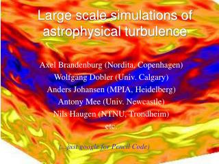
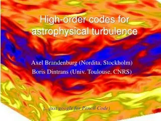
High-order codes for astrophysical turbulence Axel Brandenburg (Nordita, Stockholm) Boris Dintrans (Univ. Toulouse, CNRS) (...just google for Pencil Code)
Kolmogorov spectrum nonlinearity constant flux e [cm2/s3] [cm3/s2] E(k) a=2/3, b= -5/3 e e k
Scintillations Big Power Law in Sky • Armstrong, Cordes, Rickett 1981, Nature • Armstrong, Rickett, Spangler 1995, ApJ
Simulation of turbulence at 10243 (Porter, Pouquet,& Woodward 1998)
Direct vs hyper at 5123 Biskamp & Müller (2000, Phys Fluids 7, 4889) Normal diffusivity With hyperdiffusivity
Ideal hydro: should we be worried? • Why this k-1 tail in the power spectrum? • Compressibility? • PPM method • Or is real?? • Hyperviscosity destroys entire inertial range? • Can we trust any ideal method? • Needed to wait for 40963direct simulations
Hyperviscous, Smagorinsky, normal height of bottleneck increased Haugen & Brandenburg (PRE, astro-ph/0402301) onset of bottleneck at same position Inertial range unaffected by artificial diffusion
Bottleneck effect: 1D vs 3D spectra Why did wind tunnels not show this? Compensated spectra (1D vs 3D)
Relation to ‘laboratory’ 1D spectra Dobler, et al (2003, PRE 68, 026304)
PencilCode • Started in Sept. 2001 with Wolfgang Dobler • High order (6th order in space, 3rd order in time) • Cache & memory efficient • MPI, can run PacxMPI (across countries!) • Maintained/developed by ~40 people (SVN) • Automatic validation (over night or any time) • Max resolution so far 10243 , 4096 procs • Isotropic turbulence • MHD, passive scl, CR • Stratified layers • Convection, radiation • Shearing box • MRI, dust, interstellar • Self-gravity • Sphere embedded in box • Fully convective stars • geodynamo • Other applications • Homochirality • Spherical coordinates
Pencil formulation • In CRAY days: worked with full chunks f(nx,ny,nz,nvar) • Now, on SGI, nearly 100% cache misses • Instead work with f(nx,nvar), i.e. one nx-pencil • No cache misses, negligible work space, just 2N • Can keep all components of derivative tensors • Communication before sub-timestep • Then evaluate all derivatives, e.g. call curl(f,iA,B) • Vector potential A=f(:,:,:,iAx:iAz), B=B(nx,3)
Switch modules • magnetic or nomagnetic (e.g. just hydro) • hydro or nohydro (e.g. kinematic dynamo) • density or nodensity (burgulence) • entropy or noentropy (e.g. isothermal) • radiation or noradiation (solar convection, discs) • dustvelocity or nodustvelocity (planetesimals) • Coagulation, reaction equations • Chemistry (reaction-diffusion-advection equations) Other physics modules: MHD, radiation, partial ionization, chemical reactions, selfgravity
High-order schemes • Alternative to spectral or compact schemes • Efficiently parallelized, no transpose necessary • No restriction on boundary conditions • Curvilinear coordinates possible (except for singularities) • 6th order central differences in space • Non-conservative scheme • Allows use of logarithmic density and entropy • Copes well with strong stratification and temperature contrasts
(i) High-order spatial schemes Main advantage: low phase errors Near boundaries: x x x x x x x x x ghost zones interior points
(ii) High-order temporal schemes Main advantage: low amplitude errors 2N-RK3 scheme (Williamson 1980) 2nd order 3rd order 1st order
Evolution of code size User meetings: 2005 Copenhagen 2006 Copenhagen 2007 Stockholm 2008 Leiden 2009 Heidelberg 2010 New York
Cartesian box MHD equations Magn. Vector potential Induction Equation: Momentum and Continuity eqns Viscous force forcing function (eigenfunction of curl)
Vector potential • B=curlA, advantage: divB=0 • J=curlB=curl(curlA) =curl2A • Not a disadvantage: consider Alfven waves B-formulation A-formulation 2nd der once is better than 1st der twice!
Online data reduction and visualization non-helically forced turbulence
MRI turbulenceMRI = magnetorotational instability 2563 w/o hypervisc. t = 600 = 20 orbits 5123 w/o hypervisc. Dt = 60 = 2 orbits
Vorticity and Density See poster by Tobi Heinemann on density wave excitation!
Convection with shear and W Käpylä et al (2008) with rotation without rotation
It can take a long time Rm=121, By, 512^3 LS dynamo not always excited
Intrinsic Calculation Ray direction Transfer equation & parallelization Processors Analytic Solution:
Analytic Solution: Communication Ray direction The Transfer Equation & Parallelization Processors
Analytic Solution: Intrinsic Calculation Ray direction The Transfer Equation & Parallelization Processors
Euler potentials • Has zero magnetic helicity, A=a grad b • Strictly correct only for h=0 • Or if a and b don’t depend on the same coords
Paper arXiv:0907.1906
Roberts flow dynamo • Agreement for t<8 • For smooth fields • Not for delta-correlated • Initial fields • Exponential growth (A) • Algebraic decay (EP)
Reasons for disagreement • because dynamo field is helical? • because field is three-dimensional? • none of the two? EP too restrictive? • because h is finite?
Spurious growth for h=0 • The two agree, but are underresolved
Simple decay problem • Exponential decay for A, but not for EP!?