Download
1 / 49
500 likes | 547 Vues
Explore the Pencil Code developed by Axel Brandenburg, Wolfgang Dobler, Anders Johansen, Antony Mee, Nils Haugen, etc., for astrophysical turbulence simulations. Learn about its history, applications, high-order schemes, development issues, and more.

E N D
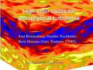
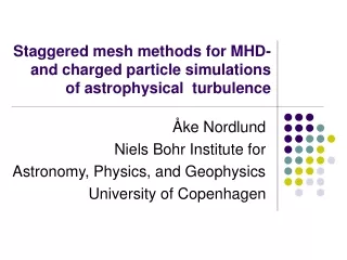
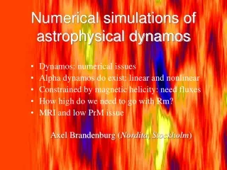
Large scale simulations of astrophysical turbulence Axel Brandenburg (Nordita, Copenhagen) Wolfgang Dobler (Univ. Calgary) Anders Johansen (MPIA, Heidelberg) Antony Mee (Univ. Newcastle) Nils Haugen (NTNU, Trondheim) etc. (...just google for Pencil Code)
Overview • History: as many versions as there are people?? • Example of a cost effective MPI code • Ideal for linux clusters • Pencil formulation (advantages, headaches) • (Radiation: as a 3-step process) • How to manage the contributions of 20+ people • Development issues, cvs maintainence • Numerical issues • High-order schemes, tests • Peculiarities on big linux clusters • Online data processing/visualization
Pencil Code • Started in Sept. 2001 with Wolfgang Dobler • High order (6th order in space, 3rd order in time) • Cache & memory efficient • MPI, can run PacxMPI (across countries!) • Maintained/developed by many people (CVS!) • Automatic validation (over night or any time) • Max resolution so far 10243 , 256 procs
Range of applications • Isotropic turbulence • MHD (Haugen), passive scalar (Käpylä), cosmic rays (Snod, Mee) • Stratified layers • Convection, radiative transport (T. Heinemann) • Shearing box • MRI (Haugen), planetesimals, dust (A. Johansen), interstellar (A. Mee) • Sphere embedded in box • Fully convective stars (W. Dobler), geodynamo (D. McMillan) • Other applications and future plans • Homochirality (models of origins of life, with T. Multamäki) • Spherical coordinates
Pencil formulation • In CRAY days: worked with full chunks f(nx,ny,nz,nvar) • Now, on SGI, nearly 100% cache misses • Instead work with f(nx,nvar), i.e. one nx-pencil • No cache misses, negligible work space, just 2N • Can keep all components of derivative tensors • Communication before sub-timestep • Then evaluate all derivatives, e.g. call curl(f,iA,B) • Vector potential A=f(:,:,:,iAx:iAz), B=B(nx,3)
A few headaches • All operations must be combined • Curl(curl), max5(smooth(divu)) must be in one go • out-of-pencil exceptions possible • rms and max values for monitoring • call max_name(b2,i_bmax,lsqrt=.true.) • call sum_name(b2,i_brms,lsqrt=.true.) • Similar routines for toroidal average, etc • Online analysis (spectra, slices, vectors)
CVS maintained • pserver (password protected, port 2301) • non-public (ci/co, 21 people) • public (check-out only, 127 registered users) • Set of 15 test problems in the auto-test • Nightly auto-test (different machines, web) • Before check-in: run auto-test yourself • Mpi and nompi dummy module for single processor machine (or use lammpi on laptops)
Switch modules • magnetic or nomagnetic (e.g. just hydro) • hydro or nohydro (e.g. kinematic dynamo) • density or nodensity (burgulence) • entropy or noentropy (e.g. isothermal) • radiation or noradiation (solar convection, discs) • dustvelocity or nodustvelocity (planetesimals) • Coagulation, reaction equations • Homochirality (reaction-diffusion-advection equations)
Features, problems • Namelist (can freely introduce new params) • Upgrades forgotten on no-modules (auto-test) • SGI namelist problem (see pencil FAQs)
High-order schemes • Alternative to spectral or compact schemes • Efficiently parallelized, no transpose necessary • No restriction on boundary conditions • Curvilinear coordinates possible (except for singularities) • 6th order central differences in space • Non-conservative scheme • Allows use of logarithmic density and entropy • Copes well with strong stratification and temperature contrasts
(i) High-order spatial schemes Main advantage: low phase errors
(ii) High-order temporal schemes Main advantage: low amplitude errors 2N-RK3 scheme (Williamson 1980) 2nd order 3rd order 1st order
Hydromagnetic turbulence and subgrid scale models? • Want to shorten diffusive subrange • Waste of resources • Want to prolong inertial range • Smagorinsky (LES), hyperviscosity, … • Focus of essential physics (ie inertial range) • Reasons to be worried about hyperviscosity • Shallower spectra • Wrong amplitudes of resulting large scale fields
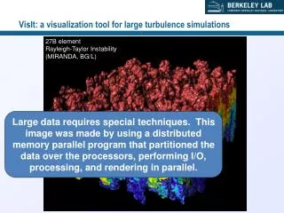
Simulations at 5123 Biskamp & Müller (2000) Normal diffusivity With hyperdiffusivity
The bottleneck: is a physical effect compensated spectrum Porter, Pouquet, & Woodward (1998) using PPM, 10243 meshpoints Kaneda et al. (2003) on the Earth simulator, 40963 meshpoints (dashed: Pencil-Code with 10243 )
Bottleneck effect: 1D vs 3D spectra Compensated spectra (1D vs 3D)
Hyperviscous, Smagorinsky, normal height of bottleneck increased Haugen & Brandenburg (PRE, astro-ph/0402301) onset of bottleneck at same position Inertial range unaffected by artificial diffusion
Structure function exponents agrees with She-Leveque third moment
Helical dynamo saturation with hyperdiffusivity for ordinary hyperdiffusion ratio 125 instead of 5
Slow-down explained by magnetic helicity conservation molecular value!!
MHD equations Magn. Vector potential Induction Equation: Momentum and Continuity eqns
Vector potential • B=curlA, advantage: divB=0 • J=curlB=curl(curlA) =curl2A • Not a disadvantage: consider Alfven waves B-formulation A-formulation 2nd der once is better than 1st der twice!
Wallclock time versus processor # nearly linear Scaling 100 Mb/s shows limitations 1 - 10 Gb/s no limitation
Sensitivity to layout onLinux clusters yprox x zproc 4 x 32 1 (speed) 8 x 16 3 times slower 16 x 8 17 times slower Gigabit uplink 100 Mbit link only 24 procs per hub
Why this sensitivity to layout? All processors need to communicate with processors outside to group of 24
Use exactly 4 columns Only 2 x 4 = 8 processors need to communicate outside the group of 24 optimal use of speed ratio between 100 Mb ethernet switch and 1 Gb uplink
Animation of energy spectra Very long run at 5123 resolution
MRI turbulenceMRI = magnetorotational instability 2563 w/o hypervisc. t = 600 = 20 orbits 5123 w/o hypervisc. Dt = 60 = 2 orbits
Homochirality: competition of left/right Reaction-diffusion equation
Conclusions • Subgrid scale modeling can be unsafe (some problems) • shallower spectra, longer time scales, different saturation amplitudes (in helical dynamos) • High order schemes • Low phase and amplitude errors • Need less viscosity • 100 MB link close to bandwidth limit • Comparable to and now faster than Origin • 2x faster withGB switch • 100 MB switches with GB uplink +/- optimal
Intrinsic Calculation Ray direction Transfer equation & parallelization Processors Analytic Solution:
Analytic Solution: Communication Ray direction The Transfer Equation & Parallelization Processors
Analytic Solution: Intrinsic Calculation Ray direction The Transfer Equation & Parallelization Processors
Current implementation • Plasma composed of H and He • Only hydrogen ionization • Only H- opacity, calculated analytically No need for look-up tables • Ray directions determined by grid geometry No interpolation is needed