Download
1 / 44
440 likes | 603 Vues
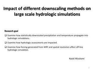
Impact of different downscaling methods on large scale hydrologic simulations. Research goal Examine how statistically downscaled precipitation and temperature propagate into hydrologic simulations. Examine how hydrologic assessments are impacted.

E N D
Impact of different downscaling methods on large scale hydrologic simulations • Research goal • Examine how statistically downscaled precipitation and temperature propagate into hydrologic simulations. • Examine how hydrologic assessments are impacted. • Examine how forcing generated from WRF and spatial resolution affect off-line hydrologic simulation. Naoki Mizukami
Outline • Background- General overview of climate data downscaling for hydrology • Part I • Comparison of model forcings • Wet-day frequency and Diurnal Temperature range • Radiation derived from downscaled climate product • Comparison of hydrologic simulations • Water balance • Extreme runoff estimations • Part II • Impacts of downscaling methods – dynamical vs. statistical • Comparison of annual cycle of forcing • Comparison of annual cycle of hydrologic fluxes and state • Impact of spatial resolutions for dynamical downscaling on hydrologic simulation • Comparison of annual cycle of hydrologic fluxes and state
Background- General overview of climate data downscaling for hydrology • For Statistical downscaled product- • Statistically downscaled estimate of wet-day frequency and extreme impact streamflow simulations (e.g. flashiness of runoff) • Other meteorological forcings (radiation and humidity) need to be estimated somehow, i.e., estimation from downscaled precipitation and temperature (i.e. MTCLM) • Radiation and humidity estimations are directly affected by precipitation (wet days) and diurnal temperature range (DTR). • Difference in radiation estimates may have significant impact on hydrologic simulation • For Dynamical downscaled product- • Spatial resolution and selection of physics used in regional weather model (e.g., WRF) affect surface meteorology, therefore hydrologic simulations.
Outline • Background- General overview of climate downscaling for hydrology • Part I • Comparison of model forcings • Wet-day frequency and Diurnal Temperature range • Radiation derived from downscaled climate product • Comparison of model simulations • Water balance • Extreme runoff estimations • Part II • Impacts of downscaling methods – dynamical vs. statistical • Comparison of annual cycle of forcing • Comparison of annual cycle of hydrologic fluxes and state • Impact of spatial resolutions for dynamical downscaling on hydrologic simulation • Comparison of annual cycle of hydrologic fluxes and state
Simulation basins PN MR CA GB UCO AR LCO RIO HUC2 HUC4 HUC8, 10, 12 are not shown Simulation focuses on western U.S. –8 HUC2 regions (shaded HUC2 domain)
Analysis: 1. Forcing 2. Water balance 3. Extreme runoff Wet day fraction (2001-2008) Mean: 0.79 Mean: 0.88 • Annual bias over CONUS • BCCA -200mm/yr • BCSDd +74mm/yr • BCSDm +30mm/yr • AR +41mm/yr Mean: 0.43 Mean: 0.34 Mean: 0.39 Gutmann et al. submitted to J.Climate
Analysis: 1. Forcing 2. Water balance 3. Extreme runoff MAM MAM JJA JJA DJF DJF SON SON Diurnal temp. range comparison (WY1980-08) Wet-day fraction comparison (WY1980-08) K fraction K
Analysis: 1. Forcing 2. Water balance 3. Extreme runoff Spatial correlation of SW radiation, wet-day fraction and DTR The upper Colorado River basin Grid boxes where Elev < 2000m • Partial rank correlation - monthly SW radiation vs. 1) wet day fraction and 2) DTR R • Overall, wet day fraction impacts SW more than DTR. • For BCSDd, majority of pixels have nearly 1.0 wet-day fraction in summer months, leading to low correlation between SW radiation and wet-day fraction. Grid boxes where Elev > 3000m R
Analysis: 1. Forcing 2. Water balance 3. Extreme runoff MAM JJA DJF SON Comparison of derived SW radiation • BCCA and BCSDd produces less SW radiation during summer compared to the others. • AR produces larger SW radiation in South-west during summer. • Difference in wet-day frequency may have more impact on SW radiation difference. W/m2 W/m2
Analysis: 1. Forcing 2. Water balance 3. Extreme runoff CLM VIC RO[mm/yr] RO[mm/yr] P[mm/yr] ET[mm/yr] ET[mm/yr] RO/P RO/P
Analysis: 1. Forcing 2. Water balance 3. Extreme runoff Comparison of precipitation partitioning PN UCO MR • Inter-comparison of S.D • All the datasets partition precipitation similarly within each region. Exception is BCCA GB AR • Inter-comparison of model • If BCCA excluded, Inter model difference is larger than inter-S.D difference especially MR, AR and UCO LCO CA RIO
Analysis: 1. Forcing 2. Water balance 3. Extreme runoff Scaling impact on extreme precipitation event over CONUS • BCSDm reproduce observed 50-yr event at all scale. • As aggregated to coarser scale, bias (e.g.BCCA and BCSDd) get smaller. Gutmann et al. submitted to J. Climate
Analysis: 1. Forcing 2. Water balance 3. Extreme runoff CLM - High flow (50yr daily maximum runoff) • Similar pattern to 50yr precipitation. • -Spatial aggregation tends to converge high extreme runoff. • - BCCA produce underestimations.
Analysis: 1. Forcing 2. Water balance 3. Extreme runoff VIC - High flow (50yr daily maximum runoff) • Similar pattern to 50yr precipitation • -Spatial aggregation tends to converge high extreme runoff
Analysis: 1.Forcing 2. Water balance 3. Extreme runoff 50yr daily maximum runoff - Inter-model comparison
Analysis: 1. Forcing 2. Water balance 3. Extreme runoff CLM - Low flow (7Q10) • Low flow extreme increase with up-scaling. (Low runoff values increase with spatial averaging)
Analysis: 1. Forcing 2. Water balance 3. Extreme runoff VIC - Low flow (7Q10 )
Analysis: 1. Forcing 2. Water balance 3. Extreme runoff 7Q10 – Inter-model comparison
Conclusions – part I Difference in statistical downscaling methods causes 1st order of difference in precipitation partitioning into runoff and ET, but inter-model difference is considerable. Choice of statistical downscaling methods impacts wet day frequency, leading to difference in shortwave radiation estimates and simulations of SWE, ET and runoff. There are substantial differences in extreme value estimates both among downscaling methods and among hydrologic models.
Outline • Background- General overview of climate downscaling for hydrology • Part I • Comparison of model forcings • Wet-day frequency and Diurnal Temperature range • Radiation derived from downscaled climate product • Comparison of model simulations • Water balance • Extreme runoff estimations • Part II • Impacts of downscaling methods – dynamical vs. statistical • Comparison of annual cycle of foricng • Comparison of annual cycle of hydrologic fluxes and state • Impact of spatial resolutions for dynamical downscaling on hydrologic simulation • Comparison of annual cycle of hydrologic fluxes and state
Comparisons (statistical downscaling methods & resolution) • Impact of downscaling methods – statistical vs. dynamical at 12km resolution Stat. downscaled Dyn. downscaled BCCA BCSDd BCSDm AR WRF Maurer 2. Impact of spatial resolutions 2.1. Dynamical downscaling WRF-4K WRF-36K WRF-12K 2.2 Statistical downscaling BCCA-6K BCSDday-6K BCSDmon-6K AR-6K BCCA-12K BCSDday-12K BCSDmon-12K AR-12K Will be included in paper Maurer – 12K Livneh – 6K
Hydrologic Simulations Hydrologic Model simulation grid (12k) Colorado Headwater analysis domain Colorado headwater WRF Simulation boundary • Simulation period : 10/2001 – 9/2008 • Model: CLM • Forcing: 4 statistical downscaled, 2 dynamical (12km raw WRF and 12km aggregated 4km WRF)
Statistical vs. Dynamical 7yr – WY2002-2008 simulation
Stat. DS vs. Dyn. DS : 1. Forcing 2. Hydrologic simulation Monthly Precipitation comparison • BCCA produces the least precipitation amount. • WRF4km aggregated precipitation is similar to Statistical downscaled data and Maurer • WRF12k precipitation is wetter in higher elevations during summer due to convective parameterization Elev. <2000m Elev. 2000m - 3000m Elev. >=3000m
Stat. DS vs. Dyn. DS : 1. Forcing 2. Hydrologic simulation Monthly SW comparison • SW from statistical downscaled and Maurer are less than WRF in lower elevation • WRF SW radiation is less in summer in high elevations compared to BCSD and Maurer Elev. <2000m Elev. 2000m - 3000m Elev. >=3000m
Stat. DS vs. Dyn. DS : 1. Forcing 2. Hydrologic simulation Monthly SWE comparison • Note scale in lowest elevation band (up to 20mm). • WRF data produce more SWE (more realistic). Ele. <2000 Ele. 2000m - 3000m Ele. >=3000m
Stat. DS vs. Dyn. DS : 1. Forcing 2. Hydrologic simulation Monthly ET comparison Elev. <2000 • ET bias pattern matches with SW radiation bias pattern in higher elevations. • WRF 12K produce high ET during summer due to high precipitation Elev. 2000 - 3000 Elev. >=3000
Stat. DS vs. Dyn. DS : 1. Forcing 2. Hydrologic simulation Monthly runoff comparison Elev. <2000 • WRF aggregated 4k produce high flow due to more SWE in high elevation RO Elev. 2000 - 3000 RO Elev. >=3000
Stat. DS vs. Dyn. DS : 1. Forcing 2. Hydrologic simulation Comparison of Precipitation partitioning • Inter-forcing difference in precipitation partitioning gets more diverse in higher elevation. • Simulations with WRF data produce higher RO ratio (and lower ET ratio) • Note difference in RO (ET) ration between WRF12km and aggregated WRF4km. ET/P or RO/P
Dynamical – 4km, 12km, and 36k 7yr – WY2001-2008 simulation
Hydrologic Simulations 36km • Model: CLM. • Analysis domain: Basin HUC 1410005 outlet: Colorado R. near Cameo. • Forcing: 4, 12, and 36km WRF 12km 4km
Dyn. DS Resolution : 1. Forcing 2. Hydrologic simulation 7yr average met. annual cycle – Colorado River near Cameo Mean Tair [K] Mean SW [W/m2] • Air Temperature- 3-4 K lower in WRF36km than 12km and 4km • SW radiation- 10-15 (5-10) W/m2 lower in WRF 4km than 36km (12km) in spring & summer
Dyn. DS Resolution : 1. Forcing 2. Hydrologic simulation 7yr average annual water cycle – Colorado River near Cameo • 36km produces greater precipitation during winter and summer • 36km produces 80mm higher SWE than 12km and 4km. • 4km produces the least ET during spring and summer possibly due to the least incoming SW • 4km produce the largest runoff. • Peak Runoff matches with simulations. Timing difference caused by snowmelt heterogeneity and subsurface processes. Observed runoff
Conclusions Part I Difference in statistical downscaling methods causes 1st order of difference in precipitation partitioning into runoff and ET, but inter-model difference is considerable. Choice of statistical downscaling methods impacts wet day fraction, leading to difference in shortwave radiation estimates and simulations of SWE, ET and runoff. There are substantial differences in extreme value estimates both among downscaling methods and among hydrologic models. Part II Winter precipitation difference affect snow accumulation. Summer precipitation differ between 4km and 12, 36km WRF (convective parameterization), but affect only low flow runoff Shortwave difference still impact on runoff.
1. Climatological comparison of model forcing Annual cycle of derived SW radiation per HUC2 region • BCCA and BCSDday tend to produce less SW during summer compared to the others
Comparison with different periods Wet days – 10/1980-9/2008 (S.D. Validation period) Wet days – 10/2000-9/2008 (S.D. Cal-Val period)
Comparison with different periods DTR – 10/1980-9/2008 (S.D. Validation period) DTR– 10/2000-9/2008 (S.D. Cal-Val period)
Comparison with different periods SW– 10/2000-9/2008 (S.D. Cal-Val period) SW – 10/1980-9/2008 (S.D. Validation period)
LW radiation – 10/1980 – 9/2008 MAM JJA DJF SON • Overall all the products are comparable. • BCCA tend to produce less LW during summer compared to the others • For LCO, all the products produce less LW than Maurer02
Relative Humidity – 10/1980 – 9/2008 MAM JJA DJF SON • BCCA tend to produce less RH throughout year compared to the others
Statistical 6km vs. 12km 7yr – WY2001-2008 simulation