Download
1 / 39
390 likes | 410 Vues
Explore Guzman's scene analysis, local and global consistency, edge detection algorithms, Laplacians, zero crossings, segmentation into regions, morphology, and Gestalt grouping in image processing. Learn about Connected Components and Vertex Categories. Understand the importance of Edge Detection in finding object boundaries and features. Discover various edge detection methods, from Frei-Chen to Laplacian, and how to handle noise sensitivity with Zero Crossings. Dive into 4-and 8-adjacency in image pixel connectivity. Enhance your knowledge in Image Understanding with practical insights and techniques.

E N D
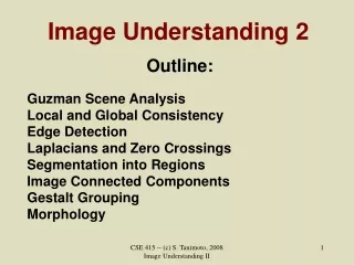
Image Understanding 2 Outline: Guzman Scene Analysis Local and Global Consistency Edge Detection Laplacians and Zero Crossings Segmentation into Regions Image Connected Components Gestalt Grouping Morphology CSE 415 -- (c) S. Tanimoto, 2008 Image Understanding II
Image Understanding 2 Outline: Guzman Scene Analysis Local and Global Consistency Edge Detection Laplacians and Zero Crossings Segmentation into Regions Image Connected Components Gestalt Grouping Morphology CSE 415 -- (c) S. Tanimoto, 2008 Image Understanding II
Blocks-World Scene Analysis(Adolfo Guzman, MIT AI Lab, 1967) • Input: a line drawing representing a 3D scene consisting of polyhedra • Output: lists of faces grouped into objects • Method: (a) classify vertices, (b) link faces according to rules, (c) extract connected components of doubly linked regions. CSE 415 -- (c) S. Tanimoto, 2008 Image Understanding II
CSE 415 -- (c) S. Tanimoto, 2008 Image Understanding II
Guzman Vertex Categories ell, arrow, fork, tee, kay CSE 415 -- (c) S. Tanimoto, 2008 Image Understanding II
Guzman Linking Rules ell, arrow, fork, tee, kay CSE 415 -- (c) S. Tanimoto, 2008 Image Understanding II
Guzman Face Grouping Criterion:Two adjacent faces must be doubly linked to be considered part of the same object. Obj1: (A B C) Obj2: (D E F G) A C B E D G F CSE 415 -- (c) S. Tanimoto, 2008 Image Understanding II
Image Understanding 2 Outline: Guzman Scene Analysis Local and Global Consistency Edge Detection Laplacians and Zero Crossings Segmentation into Regions Image Connected Components Gestalt Grouping Morphology CSE 415 -- (c) S. Tanimoto, 2008 Image Understanding II
Impossible Figures Locally consistent, globally inconsistent CSE 415 -- (c) S. Tanimoto, 2008 Image Understanding II
Image Understanding 2 Outline: Guzman Scene Analysis Local and Global Consistency Edge Detection Laplacians and Zero Crossings Segmentation into Regions Image Connected Components Gestalt Grouping Morphology CSE 415 -- (c) S. Tanimoto, 2008 Image Understanding II
Edge Detection Why? Find boundaries of objects in order to compute their features: shape, area, moments, corner locations, etc. Methods: Compute measures of change in the neighborhood of each pixel. Trace boundaries Transform each neighborhood into a vector space whose basis includes "edge" vectors. CSE 415 -- (c) S. Tanimoto, 2008 Image Understanding II
Local Edge Detectors Horizontal differences: a – b Both horiz. & vertical diffs. Roberts' cross operator (a-d)2 +(b-c)2 a b a b c d CSE 415 -- (c) S. Tanimoto, 2008 Image Understanding II
Frei-Chen Edge Detection Express each 3x3 neighborhood as a vector. N = <a, b, c, d, e, f, g, h> a b a c d e f g h CSE 415 -- (c) S. Tanimoto, 2008 Image Understanding II
Frei-Chen Edge Det. (cont) Transform it linearly into the 9D vector space spanned by the following basis vectors (each shown in 3x3 format) CSE 415 -- (c) S. Tanimoto, 2008 Image Understanding II
Image Understanding 2 Outline: Guzman Scene Analysis Local and Global Consistency Edge Detection Laplacians and Zero Crossings Segmentation into Regions Image Connected Components Gestalt Grouping Morphology CSE 415 -- (c) S. Tanimoto, 2008 Image Understanding II
Edge Finding with the Laplacian Instead of using 1st derivatives, let's consider 2nd derivatives. The Laplacian effectively finds subtle changes in intensity. 2 f(x,y) = 2 f(x,y)/x2 + 2f(x,y)/y2 discrete approximation: 0 -1 0 -1 4 -1 0 -1 0 CSE 415 -- (c) S. Tanimoto, 2008 Image Understanding II
Laplacian: Very Sensitive to Noise Remedy: First, smooth the signal with a Gaussian filter. g(x,y) = 1/(22) exp(-(x2+y2)/22 ) Then take the Laplacian. Or, directly convolve directly with a Laplacian of Gaussian (LOG). CSE 415 -- (c) S. Tanimoto, 2008 Image Understanding II
Zero Crossings The edges tend to be where the second derivative crosses 0. CSE 415 -- (c) S. Tanimoto, 2008 Image Understanding II
Zero Crossings: Example (a) orig. (b) LoG with = 1, (c) zero crossings. R Fischer et al. http://homepages.inf.ed.ac.uk/rbf/HIPR2/zeros.htm CSE 415 -- (c) S. Tanimoto, 2008 Image Understanding II
Image Understanding 2 Outline: Guzman Scene Analysis Local and Global Consistency Edge Detection Laplacians and Zero Crossings Segmentation into Regions Image Connected Components Gestalt Grouping Morphology CSE 415 -- (c) S. Tanimoto, 2008 Image Understanding II
4- and 8-adjacency If two neighboring pixels share a side, they are 4-adjacent. d's 4-adjacent neighbors are: b, c, e, g If two neighboring pixels share a corner, they are 8-adjacent d's 8-adjacent neighbors are: a,b,c,e,f,g,h a b a c d e f g h CSE 415 -- (c) S. Tanimoto, 2008 Image Understanding II
4- and 8-connectedness A set of pixels R is said to be 4-connected, provided for any pi, pj in R, there is a chain [(pi, pi' ), (pi' , pi'' ), ..., (pk, pj)] involving only pixels in R, and each pair in the chain is 4-adjacent. The chain may be of length 0. R is 8-connected, iff there exists such a chain where each pair is 8-adjacent. CSE 415 -- (c) S. Tanimoto, 2008 Image Understanding II
4- and 8-connected components 4-connected components of black: 4 8-connected components of black: 2 4-connected components of white: 2 8-connected components of white: 2 CSE 415 -- (c) S. Tanimoto, 2008 Image Understanding II
Segmentation into Regions "Dual approach" to edge detection. Let P be a digital image: P = {p0, p1, ..., pn-1} A segmentation S = {R0, R1, ..., Rm-1} is a partition of P, such that For each i, Ri is 4-connected, and Ri is "uniform", and for all i,j if Ri is adjacent to Rj, then (Ri U Rj) is not uniform. CSE 415 -- (c) S. Tanimoto, 2008 Image Understanding II
Image Understanding 2 Outline: Guzman Scene Analysis Local and Global Consistency Edge Detection Laplacians and Zero Crossings Segmentation into Regions Image Connected Components Gestalt Grouping Morphology CSE 415 -- (c) S. Tanimoto, 2008 Image Understanding II
Image Connected Components Can compute a segmentation if U(R) means all pixels in R have the same pixel value (e.g., intensity, color, etc.) Algorithm: Initialize a UNION-FIND ADT instance, with each pixel in its own subset. Scan the image. At each pixel p, check its neighbor r to the right. p and r have the same pixel value, determine whether FIND(p) = FIND(r), and if not, perform UNION(FIND(p), FIND(r)). Then check the pixel q below doing the same tests and possible UNION. When the scan is complete, each subset represents one 4-connected component of the image. CSE 415 -- (c) S. Tanimoto, 2008 Image Understanding II
Image Understanding 2 Outline: Guzman Scene Analysis Local and Global Consistency Edge Detection Laplacians and Zero Crossings Segmentation into Regions Image Connected Components Gestalt Grouping Morphology CSE 415 -- (c) S. Tanimoto, 2008 Image Understanding II
Gestalt Grouping Identification of regions using a uniformity predicate based on wider-neighborhood features (e.g., texture). CSE 415 -- (c) S. Tanimoto, 2008 Image Understanding II
Gestalt Grouping CSE 415 -- (c) S. Tanimoto, 2008 Image Understanding II
Gestalt Grouping Texture element = “texel” Texel directionality Texel granularity Alignments of endpoints Spacing of texels Groups cue for surfaces, objects. CSE 415 -- (c) S. Tanimoto, 2008 Image Understanding II
Image Understanding 2 Outline: Guzman Scene Analysis Local and Global Consistency Edge Detection Laplacians and Zero Crossings Segmentation into Regions Image Connected Components Gestalt Grouping Morphology CSE 415 -- (c) S. Tanimoto, 2008 Image Understanding II
"Mathematical Morphology" Developed at the Ecoles des Mines, France by J. Serra, from mathematical ideas of Minkowski. Idea is to take two sets of points in space and obtain a new set. Set A: the main set. Set B: the "structuring element" Set C: the result. CSE 415 -- (c) S. Tanimoto, 2008 Image Understanding II
Math. Morph. Operation 1: "Erosion" Consider each point b of B to be a vector and use it to translate a copy of A getting Ab Take the intersection of all the Ab The result is called the erosion of A by B. CSE 415 -- (c) S. Tanimoto, 2008 Image Understanding II
Erosion: example A: 0 1 1 0 0 1 1 1 0 0 0 1 1 1 0 0 0 1 0 0 B: 1 1 C: 0 0 1 0 0 0 1 1 0 0 0 0 1 1 0 0 0 0 0 0 CSE 415 -- (c) S. Tanimoto, 2008 Image Understanding II
Dilation: Take Union instead of Intersection. A: 0 1 1 0 0 1 1 1 0 0 0 1 1 1 0 0 0 1 0 0 B: 1 1 C: 0 1 1 1 0 1 1 1 1 0 0 1 1 1 1 0 0 1 1 0 CSE 415 -- (c) S. Tanimoto, 2008 Image Understanding II
Opening: Erode by B, then Dilate by –B (B rotated by ) A: 0 1 1 0 0 1 1 1 0 0 0 1 1 1 0 0 0 1 0 0 B: 1 1 C: 0 1 1 0 0 1 1 1 0 0 0 1 1 1 0 0 0 0 0 0 CSE 415 -- (c) S. Tanimoto, 2008 Image Understanding II
Closing: Dilate by B, then Erode by –B (B rotated by ) A: 0 1 1 0 0 1 1 1 0 0 0 1 1 1 0 0 0 1 0 0 B: 1 1 C: 0 1 1 0 0 1 1 1 0 0 0 1 1 1 0 0 0 1 0 0 (In this example, erosion undoes the dilation.) CSE 415 -- (c) S. Tanimoto, 2008 Image Understanding II
Closing – another example A: 0 1 1 0 0 1 0 1 0 0 0 1 0 1 0 0 0 1 0 0 B: 1 1 C: 0 1 1 0 0 1 1 1 0 0 0 1 1 1 0 0 0 1 0 0 (In this example, closing fills in holes.) CSE 415 -- (c) S. Tanimoto, 2008 Image Understanding II
Math. Morphol. Uses Repair regions corrupted by noise; Eliminate small regions Identify holes, bays, protrusions, isthmi, peninsulas, and specific shapes such as crosses. Printed circuit board inspection (find cracks, spurious wires.) Popular primitives for writing industrial machine vision apps. CSE 415 -- (c) S. Tanimoto, 2008 Image Understanding II