Chapter 8: Confidence Intervals
Chapter 8: Confidence Intervals. Lecture PowerPoint Slides. Chapter 8 Overview. 8.1 Z Interval for the Population Mean 8.2 t Interval for the Population Mean 8.3 Z Interval for the Population Proportion 8.4 Confidence Intervals for the Population Variance and Standard Deviation.


Chapter 8: Confidence Intervals
E N D
Presentation Transcript
Chapter 8:Confidence Intervals Lecture PowerPoint Slides
Chapter 8 Overview • 8.1Z Interval for the Population Mean • 8.2t Interval for the Population Mean • 8.3Z Interval for the Population Proportion • 8.4 Confidence Intervals for the Population Variance and Standard Deviation
The Big Picture Where we are coming from and where we are headed… • We stand on the threshold of the two most important statistical inference methods: confidence intervals and hypothesis testing. Everything that we have studied thus far has been in preparation for this moment. • Here in Chapter 8, we learn about confidence interval estimation, where we can infer with a certain level of confidence that our target parameter lies within a particular interval. • Every chapter from here to the end of the book will uncover a new and different topic in statistical inference. In Chapter 9, “Hypothesis Testing,” we will learn about the most prevalent method of statistical inference.
8.1: Z Interval for the Population Mean Objectives: • Calculate a point estimate of the population mean. • Calculate and interpret a Z interval for the population mean, when the population is normal, and when the sample size is large. • Find ways to reduce the margin of error. • Calculate the sample size needed to estimate the population mean.
Calculate a Point Estimate Recall that characteristics of the sample are called statistics, while characteristics of the population are called parameters. Statistical inference consists of methods for estimating and drawing conclusions about parameters, based on the corresponding statistic. Point estimation is the process of estimating unknown population parameters by known statistics. The value of each sample statistic used as an estimate is called a point estimate. Since a sample is only a small subset of a population, generalizing from a sample to the population carries the risk that the point estimate may not be very accurate. Confidence intervals help provide a means to construct an interval, based on the statistic, that is likely to contain the parameter.
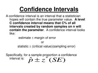
Z Interval for the Population Mean Although we cannot measure how confident we are of a statistic as a point estimate of a parameter, we can use the statistic to find an interval that is likely to contain the parameter. A confidence interval is an estimate of a parameter consisting of an interval of numbers based on a point estimate, together with a confidence level specifying the probability that the interval contains the parameter. Confidence intervals are often reported in the format: (lower bound, upper bound)
Z Interval for the Population Mean µ • The Z interval for µ may be constructed only when either of the following two conditions are met: • The population is normally distributed and σ is known. • The sample size is large (n ≥ 30), and the value of σ is known. • When a random sample of size n is taken from a population, • a (100 – α)% confidence interval is given by: • The Z interval can also be written as Z Interval for the Population Mean
Example The College Board reports that the scores on the 2010 SAT mathematics test were normally distributed. A sample of 25 scores had a mean of 510. Assume the population standard deviation is 100. Construct a 90% confidence interval for the population mean score on the 2010 SAT math test. We are 90% confident that the population mean SAT score on the 2010 mathematics SAT test lies between 477.1 and 542.9.
Margin of Error Confidence intervals for the population mean µ take the form: point estimate ± margin of error E The margin of error Eis a measure of the precision of the confidence interval estimate. For the Z interval, the margin of error takes the form E = Za/2(σ/√n). In our example, E = Za/2(σ/√n) = 32.9. Therefore, the confidence interval has the form: 510 ± 32.9 • We would like our confidence interval estimates to be as precise as possible. Therefore, we would like the margin of error to be as small as possible. There are two strategies to decrease E: • Decrease the confidence level • Increase the sample size
Sample Size for Estimating the Population Mean The sample size for a Z interval that estimates µ to within a margin of error E with confidence (100 – α)% is given by: Whenever this formula yields a sample size with a decimal, always round up to the next whole number. Sample Size for Estimating µ A natural question when constructing a confidence interval is “How large a sample size do I need to get a tight confidence interval with a high confidence level?”
8.2: t Interval for the Population Mean Objectives: • Describe characteristics of the t distribution • Calculate and interpret a t interval for the population mean.
Introducing the t Distribution In Section 8.1 we constructed confidence intervals for the population mean assuming the population standard deviation was known. In many real-world problems, we do not know the value of σ, and thus cannot use the Z interval to estimate µ. In these cases we can use s to estimate σ and use a different distribution, the t distribution. t Distribution For a normal population, the distribution of follows a t distribution, with n – 1 degrees of freedom.
Characteristics of the t Distribution • Centered at zero. The mean of t is 0, just as with Z. • Symmetric about its mean 0, just as with Z. • As df decreases, the t curve gets flatter, and the area under the t curve decreases in the center and increases in the tails. • That is, the t curve has heavier tails than the Z curve. • As df increases toward infinity, the t curve approaches the Z curve.
Finding tα/2 Step 1: Go across the row marked “Confidence level” in the t table until you find the column with the desired confidence level at the top. The tα/2 value is in this column somewhere. Step 2: Go down the column until you see the correct number of degrees of freedom on the left. The number in that row and column is the desired value of tα/2. tα/2 has area α/2 to the right of it.
Example Find the value of ta/2 that will produce a 95% confidence interval for μ if the sample size is n = 20. Step 1 Go across the row labeled “Confidence level” in the t table until we see the 95% confidence level. Step 2 df = n – 1 = 20 – 1 = 19 Go down the column until you see 19 on the left. The number in that row is ta/2 = 2.093.
t Interval for µ • The t interval for µ may be constructed when either of the following two conditions are met: • The population is normally distributed. • The sample size is large (n ≥ 30). • When a random sample of size n is taken from a population, • a (100 – α)% confidence interval is given by: • The t interval can also be written as: t Interval for the Population Mean For the t interval, the margin of error takes the form E = ta/2(s/√n). The interval can be interpreted as “We can estimate µ to within E units with (1 –a)% confidence.”
Example Use the statistics observed in Example 8.10. a. Find the margin of error for the 95% confidence interval for mean foot lengths. b. Interpret the margin of error. Solution • a. n = 20 and s = 1.280. • For a confidence level of 95%, t/2 = 2.093. • The margin of error of fourth-grade foot length is: b. We can estimate the population mean of fourth-grade foot lengths to within 0.599 centimeters with 95% confidence.
8.3: Z Interval for the Population Proportion Objectives: • Calculate the point estimate of the population proportion. • Construct and interpret a Z interval for the population proportion. • Compute and interpret the margin of error for the Z interval for p. • Determine the sample size needed to estimate the population proportion.
Calculate a Point Estimate Recall that characteristics of the sample are called statistics, while characteristics of the population are called parameters. We have dealt with interval estimates of µ, but we may also be interested in the interval estimate for the population proportion of successes, p. is a point estimate of the population proportion p.
Z Interval for the Population Proportion p Central Limit Theorem for Proportions The sampling distribution of the sample proportion follows an approximately normal distribution with mean p and standard deviation when both np ≥ 5 and n(1 – p) ≥ 5. Recall the Central Limit Theorem for Proportions We can use the CLT for Proportions to construct confidence intervals for the population proportion p.
Z Interval for the Population Proportion p The Z interval for p may be constructed only when both of the following two conditions are met: n(p-hat) ≥ 5 and n(1 – p-hat) ≥ 5. When a random sample of size n is taken from a population, a (100 – α)% confidence interval is given by: The Z interval can also be written as: Z Interval for p
Margin of Error Confidence intervals for the population proportion p take the form: point estimate ± margin of error E The margin of error Eis a measure of the precision of the confidence interval estimate. For the Z interval, the margin of error takes the form: • The margin of error E for a (1–a)% Z interval for p can be interpreted as follows: • “We can estimate p to within E with (1 –a)100% confidence.”
Example There is hardly a day that goes by without some new poll coming out. Especially during election campaigns, polls influence the choice of candidates and the direction of their policies. In October 2004, the Gallup organization polled 1012 American adults, asking them, “Do you think there should or should not be a law that would ban the possession of handguns, except by the police and other authorized persons?” Of the 1012 randomly chosen respondents, 638 said that there should NOT be such a law. a. Check that the conditions for the Z interval for p have been met. b. Find and interpret the margin of error E. c. Construct and interpret a 95% confidence interval for the population proportion of all American adults who think there should not be such a law.
Solution • Sample size is n = 1012 • Observed proportion is: • The confidence level of 95% implies that our Z/2 equals 1.96.
Solution Thus, we are 95% confident that the population proportion of all American adults who think that there should not be such a law lies between 60% and 66%.
Sample Size for Estimating the Population Proportion The sample size for a Z interval that estimates p to within a margin of error E with confidence 100(1 – α)% is given by: Whenever this formula yields a sample size with a decimal, always round up to the next whole number. When p-hat is unknown, use Sample Size for Estimating p A natural question when constructing a confidence interval is “How large a sample size do I need to get a tight confidence interval with a high confidence level?”
8.4: Confidence Intervals for the Population Variance and Standard Deviation Objectives: • Describe the properties of the c2 (chi-square) distribution, and find critical values. • Construct and interpret confidence intervals for the population variance and standard deviation.
Properties of the c2 Distribution The c2 distribution (pronounced ky-square) was discovered in 1875. The c2 random variable is continuous with the following properties: • Properties of the c2 Distribution • The total area under the curve equals 1. • The value ofc2 is never negative, so the c2 starts at 0 and extends indefinitely to the right. • The c2 curve is right-skewed. • There is a different curve for each df, n – 1. As df increases, the curve begins to look more symmetric.
c2 Critical Values To construct confidence intervals, we need to find the critical values of a c2 distribution for a given confidence level. For a confidence interval for s2 with a confidence level 100(1 – a)% we can find two critical values: • c21 -a/2= the value with area 1 – a/2 to the right of it. • c2a/2= the value with area a/2 to the right of it.
c2 Critical Values Find 20.95 and 20.05 using the 2 table and n = 10.
Confidence Interval for the Population Variance σ2 • Take a sample of size n from a normal population with mean μ and standard deviation σ. • A 100(1 – a)% confidence interval for the population variance σ2 is given by: • Where s2 represents the sample variance and 21-a/2 and 2a/2 are the critical values for a 2 distribution with n – 1 degrees of freedom.
Confidence Interval for the Population Standard Deviation σ • A 100(1 – a)% confidence interval for the population standard deviation σis then given by:
Chapter 8 Overview • 8.1Z Interval for the Population Mean • 8.2t Interval for the Population Mean • 8.3Z Interval for the Population Proportion • 8.4 Confidence Intervals for the Population Variance and Standard Deviation