Download
1 / 21
210 likes | 316 Vues
Learn how to calculate confidence intervals for a population mean using t-distributions. Understand the importance of sample size, central limit theorem, t-statistics, and interpreting t-tables.

E N D
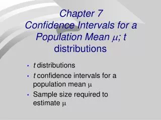
Chapter 7Confidence Intervals for a Population Mean ; t distributions t distributions t confidence intervals for a population mean Sample size required to estimate
The Importance of the Central Limit Theorem • When we select simple random samples of size n, the sample means we find will vary from sample to sample. We can model the distribution of these sample means with a probability model that is
Since the sampling model for x is the normal model, when we standardize x we get the standard normal z
If is unknown, we probably don’t know either. The sample standard deviation s provides an estimate of the population standard deviation s For a sample of size n,the sample standard deviation s is: n − 1 is the “degrees of freedom.” The value s/√n is called the standard error of x , denoted SE(x).
Standardize using s for • Substitute s (sample standard deviation) for s s s s s s s s Note quite correct Not knowing means using z is no longer correct
t-distributions Suppose that a Simple Random Sample of size n is drawn from a population whose distribution can be approximated by a N(µ, σ) model. When s is known, the sampling model for the mean x is N(m, s/√n). When s is estimated from the sample standard deviation s, the sampling model for the mean x follows at distribution t(m, s/√n) with degrees of freedom n − 1. is the 1-sample t statistic
Confidence Interval Estimates • CONFIDENCE INTERVAL for • where: • t = Critical value from t-distribution with n-1 degrees of freedom • = Sample mean • s = Sample standard deviation • n = Sample size • For very small samples (n < 15), the data should follow a Normal model very closely. • For moderate sample sizes (n between 15 and 40), t methods will work well as long as the data are unimodal and reasonably symmetric. • For sample sizes larger than 40, t methods are safe to use unless the data are extremely skewed. If outliers are present, analyses can be performed twice, with the outliers and without.
t distributions • Very similar to z~N(0, 1) • Sometimes called Student’s t distribution; Gossett, brewery employee • Properties: i) symmetric around 0 (like z) ii) degrees of freedom
Z -3 -2 -1 0 1 2 3 -3 -2 -1 0 1 2 3 Student’s t Distribution
Z t -3 -2 -1 0 1 2 3 -3 -2 -1 0 1 2 3 Student’s t Distribution Figure 11.3, Page 372
Degrees of Freedom Z t1 -3 -2 -1 0 1 2 3 -3 -2 -1 0 1 2 3 Student’s t Distribution Figure 11.3, Page 372
Degrees of Freedom Z t1 t7 -3 -2 -1 0 1 2 3 -3 -2 -1 0 1 2 3 Student’s t Distribution Figure 11.3, Page 372
t-Table: text- inside back cover • 90% confidence interval; df = n-1 = 10 0.80 0.95 0.98 0.99 0.90 Degrees of Freedom 1 3.0777 6.314 12.706 31.821 63.657 2 1.8856 2.9200 4.3027 6.9645 9.9250 . . . . . . . . . . . . 10 1.3722 1.8125 2.2281 2.7638 3.1693 . . . . . . . . . . . . 100 1.2901 1.6604 1.9840 2.3642 2.6259 1.282 1.6449 1.9600 2.3263 2.5758
Student’s t Distribution P(t > 1.8125) = .05 P(t < -1.8125) = .05 .90 .05 .05 t10 0 -1.8125 1.8125
Comparing t and z Critical Values Conf. level n = 30 z = 1.645 90% t = 1.6991 z = 1.96 95% t = 2.0452 z = 2.33 98% t = 2.4620 z = 2.58 99% t = 2.7564
Example • An investor is trying to estimate the return on investment in companies that won quality awards last year. • A random sample of 41 such companies is selected, and the return on investment is recorded for each company. The data for the 41 companies have • Construct a 95% confidence interval for the mean return.
Example • Because cardiac deaths increase after heavy snowfalls, a study was conducted to measure the cardiac demands of shoveling snow by hand • The maximum heart rates for 10 adult males were recorded while shoveling snow. The sample mean and sample standard deviation were • Find a 90% CI for the population mean max. heart rate for those who shovel snow.
EXAMPLE: Consumer Protection Agency • Selected random sample of 16 packages of a product whose packages are marked as weighing 1 pound. • From the 16 packages: • a.find a 95% CI for the mean weight of the 1-pound packages • b. should the company’s claim that the mean weight is 1 pound be challenged ?