Joint Probability Distributions
Joint Probability Distributions. Outlines Two Discrete/Continuous Random Variables Joint Probability Distributions Marginal Probability Distributions Conditional Probability Distributions Independence Multiple Discrete/Continuous Random Variables Joint Probability Distributions

Joint Probability Distributions
E N D
Presentation Transcript
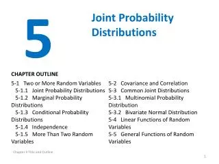
Joint Probability Distributions Outlines • Two Discrete/Continuous Random Variables • Joint Probability Distributions • Marginal Probability Distributions • Conditional Probability Distributions • Independence • Multiple Discrete/Continuous Random Variables • Joint Probability Distributions • Multinomial Probability Distribution • Covariance and Correlation • Bivariate Normal Distribution • Linear Combination of random variables
Joint Probability Distributions • In general, if X and Y are two random variables, the probability distribution that defines their simultaneous behavior is called a joint probability distribution. • For example: X : the length of one dimension of an injection-molded part, and Y : the length of another dimension. We might be interested in • P(2.95 X 3.05 and 7.60 Y 7.80).
Two Discrete Random Variables • Joint Probability Distributions • Marginal Probability Distributions • Conditional Probability Distributions • Independence
Joint Probability Distributions • The joint probability distribution of two random variables =bivariate probability distribution. • The joint probability distribution of two discrete random variables is usually written as P(X=x, Y=y).
Marginal Probability Distributions • Marginal Probability Distribution: the individual probability distribution of a random variable.
Marginal Probability Distributions • Example: The marginal probability distribution for X and Y. P(X=3)
Conditional Probability Distributions • When two random variables are defined in a random experiment, knowledge of one can change the probabilities of the other.
Conditional Mean and Variance • Example: From the previous example, calculate P(Y=1|X=3), E(Y|1), and V(Y|1).
Independence • In some random experiments, knowledge of the values of X does not change any of the probabilities associated with the values for Y. • If two random variables are independent, then
Multiple Discrete Random Variables • Joint Probability Distributions • Multinomial Probability Distribution
Joint Probability Distributions • In some cases, more than two random variables are defined in a random experiment. • Marginal probability mass function
Joint Probability Distributions • Mean and Variance
Joint Probability Distributions • Conditional Probability Distributions • Independence
Multinomial Probability Distribution • A joint probability distribution for multiple discrete random variables that is quite useful in an extension of the binomial.
Multinomial Probability Distribution • Example: Of the 20 bits received, what is the probability that 14 are Excellent, 3 are Good, 2 are Fair, and 1 is Poor? Assume that the classifications of individual bits are independent events and that the probabilities of E, G, F, and P are 0.6, 0.3, 0.08, and 0.02, respectively. • One sequence of 20 bits that produces the specified numbers of bits in each class can be represented as: EEEEEEEEEEEEEEGGGFFP • P(EEEEEEEEEEEEEEGGGFFP)= • The number of sequences (Permutation of similar objects)=
Two Continuous Random Variables • Joint Probability Distributions • Marginal Probability Distributions • Conditional Probability Distributions • Independence
Joint Probability Distributions • Example: X: the time until a computer server connects to your machine , Y: the time until the server authorizes you as a valid user. Each of these random variables measures the wait from a common starting time and X <Y. Assume that the joint probability density function for X and Y is • The probability that X<1000 and Y<2000 is:
Marginal Probability Distributions • Similar to joint discrete random variables, we can find the marginal probability distributions of X and Y from the joint probability distribution.
Marginal Probability Distributions • Example: For the random variables in the previous example, calculate the probability that Y exceeds 2000 milliseconds.
Conditional Probability Distributions • Example: For the random variables in the previous example, determine the conditional probability density function for Y given that X=x • Determine P(Y>2000|x=1500)
Conditional Probability Distributions • Mean and Variance
Conditional Probability Distributions • Example: For the random variables in the previous example, determine the conditional mean for Y given that x=1500
Independence • Example: Let the random variables X and Y denote the lengths of two dimensions of a machined part, respectively. • Assume that X and Y are independent random variables, and the distribution of X is normal with mean 10.5 mm and variance 0.0025 (mm)2 and that the distribution of Y is normal with mean 3.2 mm and variance 0.0036 (mm)2. • Determine the probability that 10.4 < X < 10.6 and 3.15 < Y < 3.25. • Because X,Y are independent
Multiple Continuous Random Variables • Marginal Probability
Multiple Continuous Random Variables • Mean and Variance • Independence
Covariance and Correlation • When two or more random variables are defined on a probability space, it is useful to describe how they vary together. • It is useful to measure the relationship between the variables.
Covariance • Covariance is a measure of linear relationship between the random variables. \ • The expected value of a function of two random variables h(X, Y ).
Covariance • Example: For the discrete random variables X, Y with the joint distribution shown in Fig. Determine
Correlation • The correlation is a measure of the linear relationship between random variables. • Easier to interpret than the covariance.
Correlation • For independent random variables
Correlation • Example: Two random variables , calculate the covariance and correlation between X and Y.
Bivariate Normal Distribution Correlation
Bivariate Normal Distribution • Marginal distributions • Dependence
Bivariate Normal Distribution • Conditional probability
Bivariate Normal Distribution Ex. Suppose that the X and Y dimensions of an injection-modeled part have a bivariate normal distribution with Find the P(2.95<X<3.05,7.60<Y<7.80)
Bivariate Normal Distribution • Ex. Let X, Y : milliliters of acid and base needed for equivalence, respectively. Assume X and Y have a bivariate normal distribution with • Covariance between X and Y • Marginal probability distribution of X • P(X<116) • P(X|Y=102) • P(X<116|Y=102)
Linear Combination of random variables • Mean and Variance
Linear Combination of random variables Ex. A semiconductor product consists of 3 layers. The variances in thickness of the first, second, and third layers are 25,40,30 nm2 . What is the variance of the thickness of the final product? Let X1, X2, X3, and X be random variables that denote the thickness of the respective layers, and the final product. V(X)=V(X1)+V(X2)+V(X3)=25+40+30=95 nm2
Homework • The time between surface finish problems in a galvanizing process is exponentially distributed with a mean of 40 hours. A single plant operates three galvanizing lines that are assumed to operate independently. • What is the probability that none of the lines experience a surface finish problem in 40 hours of operation? • What is the probability that all three lines experience two surface finish problems between 20 and 40 hours after starting the operation? • Suppose X and Y have a bivariate normal distribution with Determine the following: a) P(2.95<X<3.05) b) P(7.60<Y<7.80) c) P(2.95<X<3.05,7.60<Y<7.80)

