Download
1 / 33
330 likes | 492 Vues
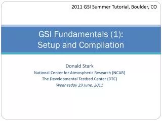
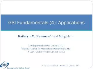
GSI Fundamentals (4): Applications. Kathryn M. Newman 1,2 and Ming Hu 1,3. 1 Developmental Testbed Center (DTC) 2 National Center for Atmospheric Research (NCAR) 3 NOAA/Global Systems Division (GSD). 2 nd On-Site GSI Tutorial Boulder, CO June 30, 2011. Outline.

E N D
GSI Fundamentals (4): Applications Kathryn M. Newman1,2and Ming Hu1,3 1Developmental Testbed Center (DTC) 2 National Center for Atmospheric Research (NCAR) 3 NOAA/Global Systems Division (GSD) 2nd On-Site GSI Tutorial Boulder, CO June 30, 2011
Outline • GSI fundamentals (1): Setup and Compilation • GSI fundamentals (2): Run and Namelist • GSI fundamentals (3): Diagnostics • GSI fundamentals (4): Applications • Where to obtain observation data • Successfully set up GSI for various data sources • Conventional observations • Radiance data • GPS RO data • Learn to check run status • Learn to understand diagnostics in the context of a particular data source • Ensure the run was successful! • This talk is tailored to Chapter 5 of the GSI User’s Guide for community release v3.0 and builds on knowledge from: ‘GSI Fundamentals (2): Run and Namelist’ & ‘GSI Fundamentals (3): Diagnostics’ Introduction| Case Study | Conventional Assimilation | Radiance Assimilation | GPS RO Assimilation | Summary
Introduction • Steps to running a successful GSI Analysis: • Obtain background field • Grab desired observational data • Modify run script to properly link observational data • Additional steps specific to observational data (e.g: thinning and bias correction for radiance) • Run GSI • Check run status and completion of each step of the GSI analysis (stdout) • Diagnose analysis results (fit files) • Check analysis increment, cost function/norm of gradient (DTC graphics utilities available) • This case study is available at: http://www.dtcenter.org/com-GSI/users/tutorial/online_tutorial/index_v3.php(practice case three) Introduction | Case Study | Conventional Assimilation | Radiance Assimilation | GPS RO Assimilation | Summary
Step 1 and 2: Case data • Cases using WRF-ARW • WRF- NMM similar • Land mask (shown below) of the background used in case study • Horizontal resolution 30-km & 51 vertical sigma levels • Background: wrfinput_<domain>_<yyyy-mm-dd_hh:mm:ss> • Obtained from the GFS forecast through WRF WPS/REAL • Real-time and archived observation data available (refer to ‘Community Tools (1): PrepBUFR/BUFR: Basic tools, NCEP data tank, and Obsproc’ for more detail) • Case Study data available at: http://www.dtcenter.org/com-GSI/users/downloads/cases/index.php Fig: Landmask of case study background Case Study : 1. background | 2. obs data | 3. run script/namelist | 4. Run | 5. stdout | 6.statistics | 7. plotting
Conventional Observation Assimilation Run Script Run Status & Completion Analysis Fit to Observations Minimization Analysis Increment Introduction | Case Study | Conventional Assimilation | Radiance Assimilation | GPS RO Assimilation | Summary
Step 3: Run Script run_gsi.ksh • Set up GSI run script following ‘GSI Run and Namelist’ talk • Set paths to data, exe, fix files, etc: Experimental Setup WORK_ROOT=/ptmp/test/gsiprd_${ANAL_TIME}_prepbufr BK_FILE=/ptmp/GSI/data/DTC/NA30km/bk/wrfinput_d01_2011-03-22_12:00:00 OBS_ROOT=/ptmp/GSI/data/DTC/NA30km/obs20110322 PREPBUFR=/ptmp/GSI/data/DTC/NA30km/obs20110322/nam.t12z.prepbufr.tm00.nr FIX_ROOT=/blhome/GSI/comGSI_v3Beta/fix CRTM_ROOT=/ptmp/GSI/CRTM/CRTM_Coefficients GSI_EXE=/blhome/GSI/comGSI_v3Beta/run/gsi.exe bk_core=ARW bkcv_option=NAM if_clean=clean • Namelist using default options in the sample script (see: GSI Fundamentals (2): Run and Namelist) Location of PREPBUFR data Conventional: 1. background | 2. obs data | 3. run script/namelist | 4. Run | 5. stdout | 6. statistics | 7. plotting
Step 4: Run Status While GSI is still running… • In ${ WORK_ROOT} contents should include: imgr_g12.TauCoeff.bin ssmi_f15.SpcCoeff.bin imgr_g13.SpcCoeff.bin ssmi_f15.TauCoeff.bin imgr_g13.TauCoeff.bin ssmis_f16.SpcCoeff.bin • Indicates CTRM coefficients linked to this run directory stdout:standard out file wrf_inout:background file gsiparm.anl: GSI namelist prepbufr:PREPBUFR file for conventional observation convinfo:data usage control for conventional data berror_stats:background error file errtable:observation error file • Indicates run scripts have successfully setup a run environment for GSI and the .exe is running. Conventional: 1. background | 2. obs data | 3. run script/namelist | 4. Run | 5. stdout | 6. statistics | 7. plotting
Step 4: Run Status While GSI is still running… • Check the content of the standard out file to monitor the stage of the GSI analysis: • be1105en% tail -fstdout 0:grepcost J,Jb,Jo,Jc,Jl = 124.503270508557578432E+04 1.150532385253925668E+03 4.388217270032186207E+04 0.000000000000000000E+00 0.000000000000000000E+00 0:grepgrad grad,reduction= 1 2 3.753613156945773994E+02 6.194241066522854222E-01 0:pcgsoi: cost,grad,step = 1 2 4.503270508557578432E+04 3.753613156945773994E+02 2.165306376032033811E-02 0:pcgsoi: gnorm(1:2),b= 8.361571469398980844E+04 8.361571469398960471E+04 5.934564861294564508E-01 0: stprat 0.106100772303380039 0: stprat 0.598874064514516721E-15 • Shows that GSI is in the optimal interation stage. 1st outer loop Inner iteration Conventional: 1. background | 2. obs data | 3. run script/namelist | 4. Run | 5. stdout | 6. statistics | 7. plotting
Step 4: Run Completion • Upon successful completion – the run directory should look like: anavinfo fort.204 l2rwbufr berror_stats fort.205 ozinfo convinfo fort.206 pcpbias_out dir.0000 fort.207 pcpinfo dir.0001 fort.208 prepbufr dir.0002 fort.209 prepobs_prep.bufrtable dir.0003 fort.210 satbias_angle errtable fort.211 satbias_in fit_p1.2011032212 fort.212 satbias_out fit_q1.2011032212 fort.213 satinfo fit_rad1.2011032212 fort.214 stdout fit_t1.2011032212 fort.215 stdout.anl.2011032212 fit_w1.2011032212 fort.217 wrf_inout fort.201 fort.220 wrfanl.2011032212 fort.202 gsi.exe fort.203 gsiparm.anl • Number of files will be greatly reduced from the run stage due to the ‘clean' option in the run script. • Important! Always check for successful completion of GSI analysis • Completion of GSI without crashing does not guarantee a successful analysis Conventional: 1. background | 2. obs data | 3. run script/namelist | 4. Run | 5. stdout | 6. statistics | 7. plotting
Step 5: Run Completionstdout: Reading in namelist • Indication GSI started normal and has read in the namelist: 0: SETUP_4DVAR: lcongrad= F 0: SETUP_4DVAR: lbfgsmin= F 0: SETUP_4DVAR: ltlint= F 0: SETUP_4DVAR: ladtest,lgrtest= F F 0: SETUP_4DVAR: lwrtinc= F 0: SETUP_4DVAR: lanczosave= F • Indication GSI is reading the background fields: 0: end_index= 348 247 50 64 0: max,min XLAT(:,1)= 13.41552734 2.813987732 0: max,min XLAT(1,:)= 47.02685928 2.813987732 0: xlat(1,1),xlat(nlon,1)= 2.813987732 4.969985962 0: xlat(1,nlat),xlat(nlon,nlat)= 47.02685928 52.26216125 0: rmse_var=XLONG ............... 0: rmse_var=U 0: ordering=XYZ 0: WrfType,WRF_REAL= 104 104 0: ndim1= 3 0: staggering= N/A 0: start_index= 1 1 1 960 0: end_index= 349 247 50 64 0: k,max,min,mid U= 1 26.24824333 -12.58862495 4.391749382 0: k,max,min,mid U= 2 27.21640015 -12.91861820 4.932917118 0: k,max,min,mid U= 3 29.04833221 -13.52361107 5.925096512 0: k,max,min,mid U= 4 32.28947067 -14.56858063 7.638842583 0: k,max,min,mid U= 5 33.57068634 -15.20958900 9.557210922 K Maximum Minimum Central grid stdout: Reading in background field Check the range of the minimum and maximum values to indicate if certain background fields are normal Conventional: 1. background | 2. obs data | 3. run script/namelist | 4. Run | 5. stdout| 6. statistics | 7. plotting
Step 5: Run Completion stdout: Reading in observational data • In the middle of the stdout file: 3:OBS_PARA: ps 2352 2572 8367 2673 3:OBS_PARA: t 4617 4331 12418 4852 3:OBS_PARA: q 3828 3908 11096 3632 3:OBS_PARA: uv 7859 6216 17360 6126 3:OBS_PARA: sst 96 239 564 150 3:OBS_PARA: pw 89 31 141 23 • This table is important to see if the observations have been read in properly Observation Type Distribution of observations in each sub-domain Conventional: 1. background | 2. obs data | 3. run script/namelist | 4. Run | 5. stdout| 6. statistics | 7. plotting
Step 5: Run Completion stdout:optimal iteration The namelist specified 2 outer loops with 50 inner loops • The optimal interation step will look as follows: 0: Minimization iteration 0 0:grepcost J,Jb,Jo,Jc,Jl = 1 0 7.447528807798134221E+04 0.000000000000000000E+00 7.447528807798134221E+04 0.000000000000000000E+00 0.000000000000000000E+00 0:grepgrad grad,reduction= 1 0 8.318335327279186231E+02 1.000000000000000000E+00 0:pcgsoi: cost,grad,step = 1 0 7.447528807798134221E+04 8.318335327279186231E+02 1.820896570337222908E-02 0:pcgsoi: gnorm(1:2),b= 3.847328648439690587E+05 3.847328648439688841E+05 5.560149119697317399E-01 0: stprat 0.989719904843960607E-01 0: stprat 0.585267682444894975E-15 • … last iteration: 0: Minimization iteration 39 0:grepcost J,Jb,Jo,Jc,Jl = 2 39 3.846412648313807586E+04 7.121785665256544235E+03 3.134234081788153344E+04 0.000000000000000000E+00 0.000000000000000000E+00 0:grepgrad grad,reduction= 2 39 7.865417003829880405E-03 3.579938402139899354E-04 0:pcgsoi: cost,grad,step = 2 39 3.846412648313807586E+04 7.865417003829880405E-03 4.600629150600819145E-02 0: PCGSOI: WARNING **** Stopping inner iteration *** 0: gnorm 0.894068220605121833E-10 less than 0.100000000000000004E-09 0: Minimization final diagnostics The iteration met the stop threshold before meeting the maximum iteration Iteration check: The J value should descend through each iteration Conventional: 1. background | 2. obs data | 3. run script/namelist | 4. Run | 5. stdout| 6. statistics | 7. plotting
Step 5: Run Completion stdout: Write out analysis results • Final step (write out results) looks very similar to section reading in background fields: 0: max,min MU= 3993.289062 -2043.328125 0: rmse_var=MU 0: ordering=XY 0: WrfType,WRF_REAL= 104 104 0: ndim1= 2 0: staggering= N/A 0: start_index= 1 1 1 0 0: end_index1= 348 247 50 1008 0: k,max,min,mid T= 1 310.9184875 233.9439850 280.6651306 0: k,max,min,mid T= 2 311.3678589 235.8090210 280.8292542 0: k,max,min,mid T= 3 311.6861572 238.1501160 281.0078125 • As an indication that GSI has successfully run – the following lines will appear at the end of the file: 0: ENDING DATE-TIME MAR 22,2011 15:52:43.541 81 TUE 2455643 0: PROGRAM GSI_ANL HAS ENDED. IBM RS/6000 SP 0:* . * . * . * . * . * . * . * . * . * . * . * . * . * . * . * . * . * . * stdout: Successful GSI run • It can be concluded GSI successfully ran through every step with no run issues. It cannot be concluded that GSI did a successful analysis until more diagnosis has been completed… Conventional: 1. background | 2. obs data | 3. run script/namelist | 4. Run | 5. stdout| 6. statistics| 7. plotting
Step 6: Analysis fit to Observations • The analysis uses the observations to correct the background fields to push the analysis results to fit the observations under certain constraints. • Easiest way to confirm the GSI analysis fit the observations better than the background? • Check fort files! • Example: fort.203 (t1) ptop 1000.0 900.0 800.0 600.0 400.0 300.0 250.0 200.0 150.0 100.0 50.0 0.0 it obs type styppbot 1200.0 999.9 899.9 799.9 599.9 399.9 299.9 249.9 199.9 149.9 99.9 2000.0 ------------------------------------------------------------------------------------------------------------------------ o-g 01 t 120 0000 count 185 529 571 988 1249 501 226 309 641 846 965 8692 o-g 01 t 120 0000 bias 0.62 0.88 -0.22 -0.19 -0.19 -0.44 -1.07 -0.97 -0.80 -1.13 -1.62 -0.92 o-g 01 t 120 0000 rms2.62 2.56 2.01 1.30 0.88 1.08 1.66 1.87 1.90 1.94 2.63 2.27 o-g 01 t 130 0000 count 0 0 0 0 0 11 177 533 67 0 0 881 o-g 01 t 130 0000 bias 0.00 0.00 0.00 0.00 0.00 0.18 0.06 -0.18 -1.23 0.00 0.00 -0.09 o-g 01 t 130 0000 rms 0.00 0.00 0.00 0.00 0.00 0.96 0.97 1.42 2.28 0.00 0.00 1.46 o-g 01 t 180 0000 count 1260 28 0 0 0 0 0 0 0 0 0 1288 o-g 01 t 180 0000 bias 0.67 0.80 0.00 0.00 0.00 0.00 0.00 0.00 0.00 0.00 0.00 0.68 o-g 01 t 180 0000 rms 1.76 1.19 0.00 0.00 0.00 0.00 0.00 0.00 0.00 0.00 0.00 1.75 o-g 01 all count 1445 557 571 988 1249 512 403 842 708 846 965 10861 o-g 01 all bias 0.67 0.87 -0.22 -0.19 -0.19 -0.42 -0.57 -0.47 -0.84 -1.13 -1.62 -0.66 o-g 01 all rms 1.89 2.51 2.01 1.30 0.88 1.08 1.40 1.60 1.94 1.94 2.63 2.16 Bias and RMS in reasonable range? – should be checked O-B Data types used: 120: rawinsonde 130: AIREP/PIREP aircraft 180: surface marine Whole atmosphere/all data: O-B – 10861 obs, bias = -0.66, rms = 1.43 Data type 120 has 1249 obs in level 400.0-599.9 mb, bias=0.19, rms =0.88 Conventional: 1. background | 2. obs data | 3. run script/namelist | 4. Run | 5. stdout | 6. statistics| 7. plotting
Step 6: Analysis fit to Observations • fort.203 (t) cont’ • Whole atmosphere, all data only: quick view of fitting • fort.202 (w) • fort.201 (p) • fort.204 (q) • Statistics show analysis results fit to obs closer than bkgd… how close analysis fit is to obs is based on ratio of bkgd error variance and observation error. o-g 01 all count 1445 557 571 988 1249 512 403 842 708 846 965 10861 o-g 01 all bias 0.67 0.87 -0.22 -0.19 -0.19 -0.42 -0.57 -0.47 -0.84 -1.13 -1.62 -0.66 o-g 01 all rms 1.89 2.51 2.01 1.30 0.88 1.08 1.40 1.60 1.94 1.94 2.63 2.16 O-B o-g 03 all count 1445 557 571 988 1249 512 403 842 708 846 965 10861 o-g 03 all bias 0.38 0.50 -0.15 -0.04 -0.01 0.04 -0.15 -0.08 0.03 -0.29 -0.31 -0.03 o-g 03 all rms 1.56 2.00 1.60 1.00 0.60 0.62 0.84 1.09 1.35 1.38 1.88 1.43 O-A Check other parameters! • 10861 total observations: from the background to the analysis the bias reduced from -0.06 to -0.03 & rms reduced from 2.16to 1.43. ~34% reduction reasonable for large scale analysis Conventional: 1. background | 2. obs data | 3. run script/namelist | 4. Run | 5. stdout | 6. statistics | 7. plotting
Step 6: Checking Minimization • In addition to stdout, GSI writes fort.220 with more detailed information on minimization • Quick check of the trend of the cost function and norm of the gradient: • Dump information from fort.220 to an output file: • be1005en% grep ‘'penalty,grad ,a,b=' fort.220 | sed -e 's/penalty,grad ,a,b=//g' > cost_gradient.txt • cost_gradient.txtwill have 6 columns (4 shown below) 0 0 0.744752880779813422E+05 0.691947026170609170E+06 1 1 0.618756484098903093E+05 0.384732864843969059E+06 1 2 0.541005432334483412E+05 0.241013229521047964E+06 1 3 0.478004546138078222E+05 0.110855305378966295E+06 1 4 0.444978275771864937E+05 0.786709661268349737E+05 1 5 0.425355924702149787E+05 0.604059171533433764E+05 … 2 35 0.384641265324412088E+05 0.432775859946986385E-03 2 36 0.384641265116106952E+05 0.292950167004207384E-03 2 37 0.384641264973069046E+05 0.197324406046192434E-03 2 38 0.384641264883406548E+05 0.107399137254121703E-03 2 39 0.384641264831380759E+05 0.618647846441362206E-04 • Both the cost function and the norm of gradient are descending with each iteration: • Cost function reduced • from 0.75 E+05 to 0.38 E+05 • Norm of gradient reduced • from 0.69 E-04 to 0.62 E-04 Norm of gradient Cost function First outer loop Inner iteration number Conventional: 1. background | 2. obs data | 3. run script/namelist| 4. Run | 5. stdout | 6. statistics| 7. plotting
Step 6: Checking Minimization • To gain a complete picture of the minimization process: plot cost function and norm of gradient • Script available under: ./util/Analysis_Utilities/plot_ncl/GSI_cost_gradient.ncl May want to change to log for easier viewing? Cost function and norm of gradient descend very fast in fist 10 iterations in both outer loops & drop slowly after the 10th iteration. Norm of gradient ascends in the second outer loop in the first several iterations Conventional: 1. background | 2. obs data | 3. run script/namelist | 4. Run | 5. stdout| 6. statistics | 7. plotting
Step 7: Checking Analysis Increment • Analysis increment gives an idea where and how much the background fields have been changed by the observations • Graphic tool available under : ./util/Analysis_Utilities/plot_ncl/Analysis_increment.ncl • The U.S. CONUS domain has many upper level observations and the data availability over the ocean is sparse Analysis Increment at the 15th Level Conventional: 1. background | 2. obs data | 3. run script/namelist | 4. Run | 5. stdout | 6. statistics| 7. plotting
Radiance Assimilation In addition to conventional: Run Script Data thinning and Bias correction Run Status & Completion Diagnosing analysis results Introduction | Case Study | Conventional Assimilation | Radiance Assimilation | GPS RO Assimilation | Summary
Step 3: Run Script run_gsi.ksh • Key difference from conventional assimilation: properly link radiance BUFR files to the GSI run directory • To add the following radiance BUFR files: AMSU-A: gdas1.t12z.1bamua.tm00.bufr_d AMSU-B: gdas1.t12z.1bamub.tm00.bufr_d HRS4: gdas1.t12z.1bhrs4.tm00.bufr_d • The location of these data is indicated in OBS_ROOT** • Insert below link to data in run_gsi.ksh: ln -s ${OBS_ROOT}/gdas1.t12z.1bamua.tm00.bufr_d amsuabufr ln -s ${OBS_ROOT}/gdas1.t12z.1bamub.tm00.bufr_d amsubbufr ln -s ${OBS_ROOT}/gdas1.t12z.1bhrs4.tm00.bufr_d hirs4bufr • Keep link to prepbufr when assimilating both prepbufr and radiance… ln -s ${PREPBUFR} ./prepbufr **To ensure correct name for radiance BUFR file, check namelist section &OBS_ROOT: dfile(30)='amsuabufr',dtype(30)='amsua',dplat(30)='n17',dsis(30)='amsua_n17',dval(30)=0.0,dthin(30)=2, • The AMSU-A observation from NOAA-17 will be read in from BUFR file ‘amsuabufr’ Radiance: 1. background | 2. obs data| 3. run script/namelist | 4. Run| 5. stdout| 6. statistics | 7. plotting
Step 3: Radiance Data Thinning • Radiance data thinning is setup in the namelist section &OBS_ROOT: • &OBS_ROOT has thinning grid array dmesh • For each data type line, the last column:‘dthin(30)=2’, is used to select the mesh grid used in the thinning. • In this case, data thinning for NOAA-17 AMSU-A observation is 60 km dmesh(1)=120.0,dmesh(2)=60.0,dmesh(3)=60.0,dmesh(4)=60.0,dmesh(5)=120 dfile(30)='amsuabufr',dtype(30)='amsua',dplat(30)='n17',dsis(30)='amsua_n17',dval(30)=0.0,dthin(30)=2, Radiance: 1. background | 2. obs data | 3. run script/namelist | 4. Run | 5. stdout | 6. statistics | 7. plotting
Step 3: Radiance Bias Correction • Radiance bias correction is very important for a successful radiance data analysis. • run_gsi.kshincludes: cp ${FIX_ROOT}/global_satangbias.txt./satbias_angle cp ${FIX_ROOT}/ndas.t06z.satbias.tm03 ./satbias_in • satbias_angletells GSI the angle bias (calculated outside GSI) • satbias_intells GSI the mass bias (calculated inside GSI from the previous cycle) The files global_satangbias.txtand ndas.t06z.satbias.tm03 can be found in ./fix for an example of bias correction coefficients. These two files should be changed with the case data or real-time data Radiance: 1. background | 2. obs data | 3. run script/namelist | 4. Run | 5. stdout | 6. statistics| 7. plotting
Step 5: Run Completion stdout: Reading in observational data • [While GSI is running] Working directory will look same as conventional, with additional links to the radiance BUFR files • Check stdout status and successful completion of each part of the analysis processes • The radiance data should have been read in and distributed to each sub domain: 3:OBS_PARA: ps 2352 2572 8367 2673 3:OBS_PARA: t 4617 4331 12418 4852 3:OBS_PARA: q 3828 3908 11096 3632 3:OBS_PARA: uv 7859 6216 17360 6126 3:OBS_PARA: sst 96 239 564 150 3:OBS_PARA: pw 89 31 141 23 3:OBS_PARA: hirs4 metop-a 0 0 28 35 3:OBS_PARA: amsua n15 2564 1333 133 195 3:OBS_PARA: amsua n18 1000 2117 0 90 3:OBS_PARA: amsuametop-a 0 0 58 67 3:OBS_PARA: amsub n17 0 0 57 70 Most radiance data read in are from AMSU-A NOAA-15 and 18 Radiance: 1. background | 2. obs data | 3. run script/namelist | 4. Run | 5. stdout| 6. statistics | 7. plotting
Step 6: Diagnosing Analysis Results • The fort.207 is statistic file for radiance data (similar to fort.203 for t) • Similar to conventional - has statistics for each outer loop: o-g 01 rad n15 amsua12805553932964718749. 19769. 1.9435 1.9435 o-g 01 rad n17 amsub 213920 254 0 0.0000 0.0000 0.0000 0.0000 … o-g 03 rad n15 amsua128055539323730910027. 10027. 0.26875 0.26875 o-g 03 rad n17 amsub 213920 254 0 0.0000 0.0000 0.0000 0.0000 • The penalty for n15 decreased from 18749 to 10027 after 2 outer loops • N17 have 213920 within the analysis time window and domain…254 after thinning…none used in analysis • When checking values: number passing quality checks similar, but final penalty smaller Penalty O-B # within the analysis time window and domain # after thinning # used in analysis O-A Statistics can also be viewed for each channel in fort.207 Radiance: 1. background | 2. obs data | 3. run script/namelist | 4. Run | 5. stdout | 6. statistics| 7. plotting
Step 7: Checking Analysis Impact • Analysis increment plotted comparing the analysis results with radiance & conventional and conventional only. • Graphic tool available under : ./util/Analysis_Utilities/plot_ncl/Analysis_increment.ncl • Impact of radiance data compared to conventional alone evident over data sparse oceans Analysis Increment at the 49th Level Increment = (AMSU-A+ PREPBUFR) - PREPBUFR Radiance: 1. background | 2. obs data | 3. run script/namelist | 4. Run | 5. stdout | 6. statistics | 7. plotting
Understanding Analysis Results • Understand the weighting functions of each channel & data coverage at the analysis time • The usage of each channel is located in the file ‘satinfo’ (see ‘GSI Fundamentals (3): Diagnostics’ for more detail) • Understand the implications of thinning • Bias correction is very important for successful radiance data analysis • Radiance bias correction for regional analysis is a difficult issue because of limited coverage of radiance data • To be considered/understood when using GSI with radiance applications Introduction | Case Study | Conventional Assimilation | Radiance Assimilation | GPS RO Assimilation | Summary
GPS RO Assimilation In addition to conventional/radiance Run Script Run Status & Completion Diagnosing analysis results Analysis Increment Introduction | Case Study | Conventional Assimilation | Radiance Assimilation | GPS RO Assimilation | Summary
Step 3: Run Script run_gsi.ksh • Key difference from conventional/radiance assimilation: properly link to GPSRO BUFR data file in the GSI run directory • The location of these data is indicated in OBS_ROOT** • Insert below link to PREPBUFR data in run_gsi.ksh: ln -s ${OBS_ROOT}/gdas1.t12z.gpsro.tm00.bufr_d gpsrobufr **To ensure correct name for GPS RO BUFR file, check namelist section &OBS_ROOT: dfile(10)='gpsrobufr',dtype(10)='gps_ref',dplat(10)='',dsis(10)='gps',dval(10)=1.0,dthin(10)=0, • In sample run script, GSI is expecting a GPS refractivity BUFR file named ‘gpsrobufr’ GPS RO: 1. background | 2. obs data | 3. run script/namelist | 4. Run | 5. stdout | 6. statistics | 7. plotting
Step 5: Run Completion stdout: Reading in observational data • While GSI is running, the working directory will look the same, with the additional links to the GPS refractivity BUFR file used • Check stdout status and successful completion of each part of the analysis processes • The GPS RO data should have been read in and distributed to each sub domain: 3:OBS_PARA: ps 2352 2572 8367 2673 3:OBS_PARA: t 4617 4331 12418 4852 3:OBS_PARA: q 3828 3908 11096 3632 3:OBS_PARA: uv 7859 6216 17360 6126 3:OBS_PARA: sst 96 239 564 150 3:OBS_PARA: pw 89 31 141 23 3:OBS_PARA: gps_ref 3538 5580 2277 6768 GPS RO refractivity data have been read in and distributed to four sub-domains successfully GPS RO: 1. background | 2. obs data | 3. run script/namelist | 4. Run | 5. stdout| 6. statistics | 7. plotting
Step 6: Diagnosing Analysis Results • The fort.212 is statistic file for GPS RO data (similar to fort.203 for t) • Statistics for each outer loop: ptop 400.0 300.0 250.0 200.0 150.0 100.0 50.0 0.0 it obs type styppbot 599.9 399.9 299.9 249.9 199.9 149.9 99.9 2000.0 ----------------------------------------------------------------------------------------- o-g 01 all count 942 675 411 496 617 853 1414 8709 o-g 01 all bias -0.11 -0.03 0.12 0.16 0.09 0.07 -0.06 -0.07 o-g 01 all rms 0.74 0.43 0.44 0.50 0.54 0.62 0.57 0.66 o-g 03 all count 95 673 413 498 629 866 1416 8890 o-g 03 all bias -0.01 -0.04 0.00 0.01 0.01 -0.01 -0.01 0.01 o-g 03 all rms 0.54 0.29 0.20 0.21 0.24 0.28 0.40 0.48 • 8709obs used in analysis during 1st outer loop, 8890 used to calculate O-A • Bias -0.07 to 0.01 after analysis. RMS 0.66 to 0.48 after analysis. O-B all GPS RO observations above 400 mb O-A GPS RO: 1. background | 2. obs data | 3. run script/namelist | 4. Run | 5. stdout | 6. statistics | 7. plotting
Step 7: Checking Analysis Impact • Analysis increment plotted comparing the analysis results with GPS RO & conventional and conventional only. • Graphic tool available under : ./util/Analysis_Utilities/plot_ncl/Analysis_increment.ncl • Impact of GPS RO data apparent over U.S. CONUS domain Analysis Increment at the 48th Level Increment = (GPS RO and PREPBUFR) - PREPBUFR GPS RO: 1. background | 2. obs data | 3. run script/namelist | 4. Run | 5. stdout | 6. statistics | 7. plotting
Summary • Steps to running a successful GSI Analysis: • Obtain background field • Grab desired observational data • Modify run script to properly link observational data • Additional steps specific to observational data (e.g: thinning and bias correction for radiance) • Run GSI • Check run status and completion of each step of the GSI analysis (stdout) • Diagnose analysis results (fit files) • Check analysis increment, cost function/norm of gradient (DTC graphics utilities available) • This case study is available at: http://www.dtcenter.org/com-GSI/users/tutorial/online_tutorial/index_v3.php(practice case three) Introduction | Case Study | Conventional Assimilation | Radiance Assimilation | GPS RO Assimilation | Summary