Manifold-Enhanced Compressive Measurement
350 likes | 458 Vues
This research highlights a significant advancement in image classification methods by leveraging manifold signal priors. By utilizing compressive measurements (CM), the proposed system enhances resilience to noise by an impressive factor of 500:1 (27 dB). The study elaborates on the structure-preserving properties of CMs and their ability to maintain geometrical relationships within sparse signal models, contributing to stable embeddings. The objectives include extending these methodologies to low-dimensional signal and task priors, leading to improved performance with reduced measurements compared to traditional techniques.

Manifold-Enhanced Compressive Measurement
E N D
Presentation Transcript
Manifold-Enhanced Compressive Measurement Richard Baraniuk Aswin Sankaranarayanan Chinmay Hegde
Research Highlight 500:1 In an image classification task, exploiting manifold signal prior improves resilience to noise by 500:1 (27dB)
Why CM Works • Compressive measurements (CMs) not full rank, but can preserve structure of signals and tasks with concise geometrical structure • sparse signal models is K-sparse • compressible signal models • “Preserves structure” = stable embedding • distances between points, angles between vectors, …
Stable Embedding (SE) An information preserving projection preserves the geometry of the set of sparse signals SE ensures that K-dim subspaces (sparse signal prior)
Our KECoM Objectives Goal: Extend to more general low-dimensional signal and task priors Metrics: Quantify progress through reduction in number of measurements (vs. Nyquist and random) for equivalent performance on a specific task K-dim subspaces
Sample Task: Classification Simple object classification problem AWGN: nearest neighbor classifier Common issue: L unknown articulation parameters Common solution: matched filter find nearest neighbor under all articulations
Matched Filter Geometry Classification with L unknown articulation parameters Images are points in Classify by finding closesttarget template to datafor each class distance or inner product optimal under AWGN model data target templatesfromgenerative modelor training data (points)
Matched Filter Geometry Classification with L unknown articulation parameters Images are points in Classify by finding closesttarget template to data As template articulationparameter changes, points map out a L-dimnonlinear manifold Matched filter classification = closest manifold search data articulation parameter space
Manifold Signal Prior • translations of an object • q: x-offset and y-offset q2Q Our interest here: Collections of “images” parameterized by
Manifold Signal Prior • translations of an object • q: x-offset and y-offset • wedgelets • q: orientation and offset q2Q Our interest here: Collections of images parameterized by
Manifold Signal Prior • translations of an object • q: x-offset and y-offset • wedgelets • q: orientation and offset • rotations of a 3D object • q: pitch, roll, yaw q2Q Our interest here: Collections of images parameterized by
Manifold Signal Prior • translations of an object • q: x-offset and y-offset • wedgelets • q: orientation and offset • rotations of a 3D object • q: pitch, roll, yaw q2Q • Image articulation manifold Our interest here: Collections of images parameterized by
Manifold Task Priors L-dim manifolds To preserve structure of classification task, stably embed joint manifold comprising the various target classes
Whitney’s (Easy) Embedding Theorem • THEOREM (1936) Let F be a compact Hausdorff CrL-dimensional manifold with r>2. Then there is a Crembedding of F in R2L+1 • Glossary • compact: closed and bounded (in RN) • Hausdorff: different points have different neighborhoods • Cr: charts are differentiable • embedding: one-to-one mapping (not necessarily onto) • Upshot: only 2L+1 compressive measurements necessary to solve classification problem
KECoM Matched Filter Take M>2L+1 compressive measurements of scene and perform classification in compressed domain
Key Insight from WET Proof[Hirsch, Kirby ‘99] • Suppose we have an L-dimensional manifold in Rq, with q > 2L+1 • try to project everything to Rq-1 • Construct set S of secants • each is a direction not to project • S is (2K)-dimensional • does not fillSq-1 (since q-1 > 2L) • Choose an admissible projection from Sq-1 • new manifold is embedded in Rq-1 (no overlaps) • Repeat until dimension 2L+1
Key Insight from WET Proof[Hirsch, Kirby ‘99] • Suppose we have an L-dimensional manifold in Rq, with q > 2L+1 • try to project everything to Rq-1 • Construct set S of secants • each is a direction not to project • S is (2K)-dimensional • does not fillSq-1 (since q-1 > 2L) • Upshot: compressive measurement directions are orthogonal to secant set • compute via PCA of secant set • dependent on both signal priors and task prior
Example 1: Manifold Learning • Truck traveling along roadway, L=2 • Noise added to images • Goal: Learn dimensionality of manifold task prior • N = 90 x 120 = 10800 pixels • M = 60 compressive measurements (180:1 compression) • 540 training images M=60KECoM M=60random clean image noisy image M=10800
Example 2: Recovery test image measurements CoM project onto manifold CoM adjoint Goal: Quantify ability of compressive measurements to capture essence of a manifold signal prior Metric: Recovery SNR of adjoint of measurement operator Compare: Manifold-adaptive to random measurements
Example 2: Recovery random measurement adjoint measurement vectors learned by PCA on secant set test image PCA-secant adjoint • Goal: Quantify (in terms of SNR) ability of compressive measurements to capture essence of a manifold signal prior • 200 images from a 2-D translation manifold • N = 128x128 = 16384 pixels • 200*199/2 secants • truncated SVD yields M=30 measurement vectors (546:1 compression)
Example 2: Recovery random measurement adjoint measurement vectors learned by PCA on secant set test image PCA-secant adjoint • Goal: Quantify (in terms of SNR) ability of compressive measurements to capture essence of a manifold signal prior • 200 images from a 2-D translation manifold • N = 128x128 = 16384 pixels • 200*199/2 secants • truncated SVD yields M=30 measurement vectors (546:1 compression)
Example 2: Recovery SNR performance as a function of number of measurements square circle • Goal: Quantify (in terms of SNR) ability of compressive measurements to capture essence of a manifold signal prior • 200 images from a 2-D translation manifold • N = 128x128 = 16384 pixels • 200*199/2 secants • truncated SVD yields M=30 measurement vectors (546:1 compression)
Example 3: Classification • Classification requires measurement vectors that preserve inter-class variations • Joint: - learn PCA-secants on data from both classes jointly - supports both image recovery and classification • Inter-class: - learn PCA-secants on the inter-class secants - supports classification but not recovery test images inter-class joint
Example 3: Classification • Classification requires measurement vectors that preserve inter-class variations • Joint: - learn PCA-secants on data from both classes jointly - supports both image recovery and classification • Inter-class: - learn PCA-secants on the inter-class secants - supports classification but not recovery Conclusion: relaxingtask from recovery toclassification improvesperformance Prob correct classification number of measurements
Example 3: Classification • Classification requires measurement vectors that preserve inter-class variations • Joint: - learn PCA-secants on data from both classes jointly - supports both image recovery and classification • Inter-class: - learn PCA-secants on the inter-class secants - supports classification but not recovery Number of measurements = 20 Number of measurements = 30
Example 4: Classification • Class 1/2: Truck with/without payloadTrucks traveling along roadway, L=2 • Study: Robustness of classification wrt noise added to images • N = 240 x 320 = 76800 pixels • M = 80 compressive measurements (960:1 compression) • 30 training images from each class • 200 test images 500:1 (27dB)
Example 5: Classification on MSTAR T72 BTR70 BMP2 • Training data: 230 data points per class • Test dataset: 190 data points per class • Manifold signal priors • no analytical projection onto manifold • solution: SVM classifier
Example 5: Classification on MSTAR Measurement vectors learned by PCA on secant set (inter-manifold)
Example 5: Classification on MSTAR • Training data: 230 data points per class • Test dataset: 190 data points per class • Manifold signal priors • no analytical projection onto manifold • solution: SVM classifier
Research Directions (1/3) • Derive necessary and sufficient conditions for stable embedding and compare to random projection approach (CS/Johnson-Lindenstrauss) • Exploit analytical structure of special manifolds • ex: Lie groups (affine transformations) • analytical characterization of secant set • fast algorithms for measurement design/adaptation? • Alternatives to classical secants for different tasks • ex: for classification only need embedding to preserve inter-manifold distances and not intra-manifold distances • weight secants according to their contribution to a task-specific metric (ex: classifier margin)
Research Directions (2/3) • Practical realities of radar imaging • High dynamic range of radar images • corner reflector glints, … • Support active sensing • implementation in a radar system requires convolutional structure in manifold-secant measurement vectors
Research Directions (3/3) • Non-differentiability of image manifolds • no embedding guarantee • difficult to navigate • One solution: progressively smooth manifold (coarse-to-fine) by blurring imagery [Wakin, Donoho, Choi, B] • Points toward multiscale compressive measurements • explore ties with Rice model-based CM