Capacity
Capacity. After deciding what products/services should be offered and how they should be made, management must plan the capacity of its processes.

Capacity
E N D
Presentation Transcript
Capacity After deciding what products/services should be offered and how they should be made, management must plan the capacity of its processes. Capacity is the maximum rate of output for a process. Must have capacity to meet current and future demands. Long-term capacity plans deal with investments in new facilities and equipment. Short-term capacity plans focus on workforce size, overtime budgets, and inventories.
Capacity Planning • This activity is central to the long-term success of an organization. • Too much capacity can be as problematic as too little • Capacity planning considers questions such as: • How much of a cushion is needed? • Should we expand capacity before the demand is there or wait until demand is more certain?
Capacity Planning • Capacity can be defined as the ability to hold, receive, store, or accommodate. • Strategic capacity planning is an approach for determining the overall capacity level of capital intensive resources, including facilities, equipment, and overall labor force size.
Measuring capacity • No single capacity measure is universally applicable. • Capacity can be expressed in terms of outputs or inputs. • Output measures—the usual choice for line flow processes, usually high-volume • Low amount of customization • Product mix becomes an issue when the output is not uniform in work content. • Input measures—used for flexible flow, low-volume processes • High amount of customization • Output varies in work content; a measure of total units produced is meaningless. • Output is converted to some critical homogeneous input, such as labor hours or machine hours.
Average output rate Peak capacity Utilizationpeak = Average output rate Effective capacity Utilizationeffective = Utilization Fabrication can make 100 engines/day Management wants 45 engines/day Currently producing 50 engines/day x 100% x 100%
Utilization Fabrication can make 100 engines/day Management wants 45 engines/day Currently producing 50 engines/day 50 100 Utilizationpeak = x 100% = 50% 50 45 Utilizationeffective = x 100% = 111% The average output rate and the capacity must be measured in the same terms.
Types of Capacity • Peak capacity • Calling for extraordinary effort under ideal conditions that are not sustainable • Allows for downtime for maintenance and repair. • Engineering assessment of maximum annual output • Effective capacity • Economically sustainable under normal conditions
Utilization What does it mean? Even through the department falls well short of peak capacity, it is well beyond the output rate judged to be most economical. It’s operations could be sustained at that level only through the use of considerable overtime; capacity expansion should be evaluated.
Utilization Capacity cushion – amount of reserve capacity that a firm maintains to handle sudden increases in demand or temporary loss of production capacity. Utilizationpeak = 50% Utilizationeffective = 111% Capacity cushionpeak = 100% – 50% = 50% Capacity cushioneffective = 100% – 111% = – 11%
Best Operating Level Best Operating Level Average unit cost of output Underutilization Overutilization Volume
To customers Inputs 1 2 3 200/hr 200/hr 50/hr (a) Operation 2 a bottleneck Capacity Bottlenecks “A bottleneck is an operation that has the lowest effective capacity of any operation in the facility and thus limits the system’s output.”
To customers Inputs 1 2 3 200/hr 200/hr 200/hr Capacity Bottlenecks (b) All operations bottlenecks In effect, the process can produce only as fast as the slowest operation. True expansion of a process’s capacity occurs only when bottleneck capacity is increased. In the first slide, adding capacity at Operation 1 or 3 will not impact system capacity. However, when adding capacity to Operation 2, must then increase capacity at all 3 operations to increase capacity further. To increase capacity: new equipment, new facilities, expanded operating hours, increased shifts, increased work hours, or redesign the process
Theory of Constraints • Focus is on whatever impedes, (i.e., bottlenecks) progress toward the goal of maximizing flow of total value-added funds (sales less discounts and variable costs) • The focus on bottlenecks is the means to increase throughput and, consequently, the flow of value added funds. • The performance of the overall system is a function of how bottleneck operations or processes are scheduled.
Theory of Constraints • Short-term: overtime, temporary employees, outsource • Increase effective capacity utilization at bottlenecks without experiencing the higher costs and poor customer service usually associated with maintaining output rates at peak capacity. • Carefully monitor short-term schedules, minimize idle time, setups (changes from one product to another).
Theory of Constraints Identify the system bottleneck(s) Exploit the bottleneck(s) Subordinate all other decisions to step 2 Elevate the bottleneck(s) Do not let inertia set in
Economies of Scale • Increasing output rate decreases the average unit cost • Fixed costs are spread over more units • Construction costs are reduced • Costs of purchased materials are cut • Process advantages are found
Diseconomies of Scale • When the average costs per unit increases as the facility’s size increases. • Excessive size can bring complexity, loss of focus, and inefficiencies, which raise the average unit cost. • Characterized by loss of agility, less innovation, risk avoidance, and excessive analysis and planning at the expense of action. • Nonlinear growth of overhead leads to employee ceilings.
Economies and Diseconomies of Scale Best operating level is 500-beds; optimal depends on number of patients per week. 250-bed hospital 750-bed hospital 500-bed hospital Average unit cost (dollars per patient) Economies of scale Diseconomies of scale Output rate (patients per week)
Capacity strategy • Sizing capacity cushions • Average utilization rates near 100% indicate: • Need to increase capacity • Poor customer service or declining productivity • Utilization rates tend to be higher in capital-intensive industries.
Capacity Strategy • Factors Leading to Large Capacity Cushions • When demand is variable, uncertain, or product mix changes • When finished goods inventory cannot be stored • When customer service is important • When capacity comes in large increments • When supply of material or human resources is uncertain • Factors leading to small capacity cushions • Unused capacity costs money. • Large cushions hide inefficiencies, absenteeism, unreliable material supply. • When subcontractors are available to handle demand peaks
Capacity Strategy • Timing and sizing of expansion • Expansionist strategy • Keeps ahead of demand, maintains a capacity cushion • Large, infrequent jumps in capacity • Higher financial risk • Lower risk of losing market share • Economies of scale may reduce fixed cost per unit • May increase learning and help compete on price • Preemptive marketing
Capacity Strategy • Wait-and-see strategy • Lags behind demand, relying on short-term peak capacity options (overtime, subcontractors) to meet demand • Lower financial risk associated with overly optimistic demand forecast • Lower risk of a technological advancement making a new facility obsolete • Higher risk of losing market share • Follow-the-leader strategy • An intermediate strategy of copying competitors’ actions • Tends to prevent anyone from gaining a competitive advantage
Capacity Strategies Forecast of capacity required Planned unused capacity Capacity increment Capacity Time between increments Time (a) Expansionist strategy
Capacity Strategies Forecast of capacity required Planned use of short-term options Capacity increment Capacity Time between increments Time (b) Wait-and-see strategy
Linking Capacity and Other Decisions • Competitive Priorities • Quality Management • Capital Intensity • Resource Flexibility • Inventory • Scheduling
Item Client X Client Y Annual demand forecast (copies) 2000.00 6000.00 Standard processing time (hour/copy) 0.50 0.70 Average lot size (copies per report) 20.00 30.00 Standard setup time (hours) 0.25 0.40 [Dp + (D/Q)s]product 1 + ... + [Dp + (D/Q)s]product n N[1 – (C/100)] M = Capacity Decisions Estimate Capacity Requirements
Item Client X Client Y Annual demand forecast (copies) 2000.00 6000.00 Standard processing time (hour/copy) 0.50 0.70 Average lot size (copies per report) 20.00 30.00 Standard setup time (hours) 0.25 0.40 [2000(0.5) + (2000/20)(0.25)]client X + [6000(0.7) + (6000/30)(0.4)]client Y (250 days/year)(1 shift/day)(8 hours/shift)(1.0 – 15/100) M = Capacity Decisions Estimate Capacity Requirements
Item Client X Client Y Annual demand forecast (copies) 2000.00 6000.00 Standard processing time (hour/copy) 0.50 0.70 Average lot size (copies per report) 20.00 30.00 Standard setup time (hours) 0.25 0.40 5305 1700 M = = 3.12 4 machines Capacity Decisions Estimate Capacity Requirements Example 8.2
Kitchen Capacity Gaps Year 1: 90,000 – 80,000 = 10,000 Year 2: 100,000 – 80,000 = 20,000 Year 3: 110,000 – 80,000 = 30,000 Year 4: 120,000 – 80,000 = 40,000 Year 5: 130,000 – 80,000 = 50,000 Demand Year 1: 90,000 meals Year 2: 100,000 meals Year 3: 110,000 meals Year 4: 120,000 meals Year 5: 130,000 meals Capacity Decisions Identify Capacity Gaps Kitchen capacity = 80,000 meals Dining room capacity = 105,000 meals
Dining Room Capacity Gaps Year 1: no gaps Year 2: no gaps Year 3: 110,000 – 105,000 = 5,000 Year 4: 120,000 – 105,000 = 15,000 Year 5: 130,000 – 105,000 = 25,000 Demand Year 1: 90,000 meals Year 2: 100,000 meals Year 3: 110,000 meals Year 4: 120,000 meals Year 5: 130,000 meals Capacity Decisions Identify Capacity Gaps Kitchen capacity = 80,000 meals Dining room capacity = 105,000 meals
Year Demand Cash Flow 1 90,000 (90,000 – 80,000)2 = $20,000 2 100,000 (100,000 – 80,000)2 = $40,000 3 110,000 (110,000 – 80,000)2 = $60,000 4 120,000 (120,000 – 80,000)2 = $80,000 5 130,000 (130,000 – 80,000)2 = $100,000 Capacity Decisions Evaluate Alternatives Expand capacity to meet expected demand through Year 5
Capacity Decisions Evaluate Alternatives
TIME TO PERFORM (SECONDS) Standard OPERATION Average Deviation Review renewal application for correctness 15 3 Check file for violations and restrictions 60 15 Process and record payment 25 6 Conduct eye test 35 10 Photograph applicant 20 5 Issue temporary license 30 5 AVERAGE CUSTOMER ARRIVAL TIME (PEOPLE PER MINUTE) 8:00 A.M. — 9:00 A.M. 1.25 9:00 A.M. — 12:00 P.M. 0.75 12:00 P.M. — 1:00 P.M. 2.00 1:00 P.M. — 4:00 P.M. 0.75 Capacity Decisions Simulation
Capacity Decisions Bottleneck
Capacity Decisions Bottleneck