Ch. 5 Data Encoding
Ch. 5 Data Encoding. Ch. 5 Data Encoding. 5.1 Digital Data, Digital Signals 5.2 Digital Data, Analog Signals 5.3 Analog Data, Digital Signals 5.4 Analog Data, Analog Signals. Introduction to Ch. 5. Figure 5.1--Encoding and Modulation Techniques Encoding onto a digital signal--x(t)

Ch. 5 Data Encoding
E N D
Presentation Transcript
Ch. 5 Data Encoding • 5.1 Digital Data, Digital Signals • 5.2 Digital Data, Analog Signals • 5.3 Analog Data, Digital Signals • 5.4 Analog Data, Analog Signals
Introduction to Ch. 5 • Figure 5.1--Encoding and Modulation Techniques • Encoding onto a digital signal--x(t) • Digital or analog source--g(t) • Modulation onto an analog signal--modulated signal s(t) • Digital or analog source--modulating signal m(t) • Four Possible Combinations • Data Source: Analog or Digital • Signal Transmission: Analog or Digital
5.1 Digital Data, Digital Signals: Terminology • A digital signal is a sequence of discrete, discontinuous voltage pulses. • Each pulse is a signal element. • Signal elements can be unipolar or bipolar.
5.1 Digital Data, Digital Signals: Terminology (p.2) • The data rate is the number of bits per second being transmitted--R bps. • The duration of a bit (or one bit time) is 1/R for binary signaling. • The signaling rate or modulation rate (baud rate) is the number of signal elements per second. • A mark refers to a logic 1 and a space refers to a logic 0.
5.1 Digital Data, Digital Signals--The Encoding Scheme • The encoding scheme is the mapping from data bits to signal elements. • Evaluation of encoding schemes. • Does the encoding effectively use the spectrum? • Does the encoding scheme support synchronization (clocking)? • Does the encoding permit errors to be detected more quickly? • Is the encoding scheme resistant to noise? • How costly and complex is the scheme?
5.1 Digital Signal Encoding Formats • Nonreturn-to-Zero • NRZ-L (Level) • NRZI (Invert on Ones) • Multilevel Binary • Bipolar-AMI (Alternate Mark Inversion) • Pseudoternary • Biphase • Manchester • Differential Manchester
5.1 Tables and Figures • Table 5.2--Definition of Digital Signal Encoding Formats • Figure 5.2--Digital Signal Encoding Formats (waveforms) • Figure 5.3--Spectral Density of Various Signal Encoding Schemes (illustrates bandwidths) • Figure 5.4--Theoretical Bit Error Rate for Various Digital Encoding Schemes (noise immunity)
5.1 Nonreturn to Zero (NRZ) • Two different voltage levels are used to represent a 0 and a 1. • The voltage level remains constant throughout the bit interval. • NRZ-L (Nonreturn to Zero--Low) • Binary 0-- high voltage. • Binary 1-- low voltage.
5.1 Nonreturn to Zero (NRZ) (p.2) • NRZI (Nonreturn to zero--Invert on 1’s) • Binary 0--no transition. • Binary 1--a transition (high-to-low or low-to-high) at the beginning of the bit interval. • Differential encoding--the signal is decoded by comparing the polarity of adjacent signal elements (eg. NRZI).
5.1 Evaluating NRZ • Signal Spectrum--Efficient use of bandwidth; but there is a DC component. • Clocking--no special synchronization capability. • Error Detection--no special error detection capability. • Signal Interference and Noise Immunity--bit error rate performance is better than multilevel binary (at a given S/N ratio.) • Cost and Complexity--simple and easy to engineer.
5.1 Evaluating NRZ (p.2) • Summary • Commonly used for digital magnetic recording. • Other techniques are often better for transmission.
5.1 Multilevel Binary • More than two signal levels • Bipolar-AMI • Binary 0 -- no pulse. • Binary 1 -- positive or negative pulse, alternating for successive ones. • Pseudoternary • Binary 0 --positive or negative pulse, alternating for successive 0's. • Binary 1 --no pulse.
5.1 Evaluating Multilevel Binary • Signal Spectrum • No DC component. • Less bandwidth is required than for NRZ. • Clocking • Some synchronization capability. • Bipolar-AMI is sensitive to strings of 0's and pseudoternary is sensitive to strings of 1's. • Error Detection • Some errors can be detected when pulse alternation property is violated.
5.1 Evaluating Multilevel Binary (p.2) • Signal Interference and Noise Immunity • Not as good as NRZ. • Cost and Complexity • More complex than NRZ. • Summary • Variations are used for long distance communications and ISDN.
5.1 Biphase • Manchester (LAN Standards) • A transition occurs in the middle of each bit period. • Binary 1--low-to-high transition. • Binary 0--high-to-low transition. • Differential Manchester • Beginning of the bit period is important. • Binary 0 --transition at the beginning of a bit period. • Binary 1-- no transition at the beginning of a bit period. • The mid-bit transition is only for clocking.
5.1 Evaluating Biphase • Signal Spectrum • No DC component. • Large bandwidth requirement. • Clocking • Self-clocking--always a transition in the middle of each bit. • Error Detection • The absence of an expected transition can be used to detect errors.
5.1 Evaluating Biphase (p.2) • Signal Interference and Noise Immunity • Same as NRZ and better than multilevel binary (for a given S/N ratio). • Cost and Complexity--complex. • Summary • Manchester is used for IEEE 802.3 (Ethernet). • Differential Manchester is used in IEEE 802.5 (token ring).
5.1 Modulation Rate vs. Data Rate • Let R be the data rate or bit rate (bps) • Let D be the rate at which signal elements are generated (signaling rate) in baud (signals/sec.). • Let M be the number of signal elements. • Let L be the number of bits per signal element--L = log2(M). • Then: R = D (signals/sec) x L (bits/signal) • Note: Some authors differ from Stallings.
5.1 Scrambling Techniques • Problem: Long strings of 1’s or O’s could cause difficulty in clocking. • Solution: Substitute signals with transitions for those with none. • Bipolar with 8-zeros substitution (B8ZS) • Based on bipolar-AMI (North America.) • 8 0's replaced by string with 2 code violations. • High -density bipolar --3 zeros (HDB3) • Based on bipolar-AMI (Europe and Japan.) • 4 0's replaced by string with 1 code violation.
5.2 Digital Data, Analog Signals --Modulation Techniques • Amplitude-shift keying (ASK) (Fig. 5.7) • Binary 1: s1(t)= A cos(2pfct) • Binary 0: s0(t)= 0 • Susceptible to additive noise. • Somewhat inefficient as related to bandwidth. • Used with optical fibers (low and high amplitudes, A0 and A1.)
5.2 Modulation Techniques (p.2) • Binary Frequency-Shift Keying (BFSK) • Binary 1: A cos(2pf1t) • Binary 0: A cos(2pf2t) • Fig. 5.8 shows full duplex BFSK transmission on a voice grade line--Bell System 108 modems. • Bandwidth is split at 1700 Hz. • One direction has frequencies at 1170 +/- 100Hz. • The other has frequencies at 2125+/- 100 Hz. • BFSK is less susceptible to errors than ASK.
5.2 Modulation Techniques (p.3) • Multiple FSK (MFSK) • There are M signal elements. • si(t)= A cos(2pfit), 1 i M (Eq. 5.4) • fc = the carrier frequency • fd = the difference frequency • M = number of signal elements • L = number bits encoded in a signal element • fi = fc + (2i-1 -M) fd
5.2 Modulation Techniques (p.4) • MFSK (cont.) • Signal is held for a period of Ts= LT where T is the bit time. • Bandwidth required is 2Mfd=M/Ts • Minimum frequency spacing is 2fd. • See Fig. 5.9 for an example with M =4.
5.2 Modulation Techniques (p.5) • Example 5.1 MFSK (M=8) • fc=250 kHz, fd=25kHz, M = 8 (L = 3) • f1 = 250 k Hz + (2x1 - 1 - 8) x 25kHz • = 250 k Hz + (-7) x 25 k Hz = 75 k Hz. • See page 144 for f2, ..., f8. • Data rate of 2fd = 1/Ts = 50 k bps can be supported. • Bandwidth of Wd=2Mfd=400 k Hz.
5.2 Modulation Techniques (p.6) • Two-Level Phase-Shift Keying (BPSK) • Binary 1: A cos(2pfct) = (+1) A cos(2pfct) • Binary 0: A cos(2pfct + p)= (-1) A cos(2pfct) • Alternative Representation for (BPSK) • Let d(t) be a signal that takes on the values of +1 and -1. • sd(t) = A d(t) cos(2pfct) (Eq. 5.6)
5.2 Modulation Techniques (p.7) • Differential PSK (DPSK) (Fig. 5.10) • Binary 0: send a signal burst same as the previous signal burst. • Binary 1: send a signal burst of opposite phase as the previous burst (change by p degrees.) • Multiple signaling is possible. • Ex.1QPSK--4 angles; 2 bits per signal. (Eq. 5.7) • Ex.2: Standard 9600 bps transmission. • 16 signals with 4 bits per signal. • 3 different amplitudes. • 12 different angles (some angles have 2 amplitudes.)
5.2 Data Rate (R) vs. Signaling Rate (D) • Recall: R = D x L = D x log2 (M). • D = the signaling rate (or modulation rate) in bauds. • M = the number of signal elements. • L= the number of bits per signal element. • Example : Standard 9600 bps Modem • D = 2400 signals/sec (baud). • M=16 signal elements. • L= log2 (16)= 4 bits/signal element. • R= 2400 x 4= 9600 bps.
5.2 Performance of Digital Modulation Schemes • Transmission bandwidth requirements. • ASK: BT = (1 + r) R (Eq. 5.8) • R is the bit rate and "r" is related to the filtering technique used, and 0 < r < 1. • FSK: BT = 2DF + (1+r)R (Eq. 5.9) • DF = the offset of the modulated frequency from the carrier frequency. • MPSK: BT = (1 +r) R /[log2(M)] (Eq. 5.10) • MFSK: BT = (1+r)MR /[log2(M)] (Eq. 5.11) • Note: For digital signaling, BT = .5(1+r)D.
5.2 Performance of Digital Modulation Schemes (p.2) • Table 5.5 shows R/BT (bandwidth efficiency.) • ASK: R/ BT =1 / (1 + r) • FSK: R/ BT =1 / [2)F/R + (1+r)] • PSK: R/ BT = 1/ (1 +r) • Multilevel PSK: R/ BT = [log2(M)] / (1+r) • NOTE: Multilevel signaling increases bandwidth efficiency above 1. • NOTE2: Table 5.5 notation: M=L; L=b (edition 6 notation--needs editing.)
5.2 BER Performance and Bandwidth Efficiency • Figure 5.4--BER as a function of Eb/No. • PSK/QPSK performs 3dB better than ASK/FSK. • If we increase Eb/No then we decrease BER. • Recall that Eb =STb, Tb = 1/R. • Then Eb/No= STb / No = S/(No x R). • Fig. 5.13--FSK and MPSK BER vs. Eb/No • So to improve the BER performance • Increase signal strength (increase S/N). • Decrease R, which actually increases Eb.
5.2 BER Performance and Bandwidth Efficiency (p.2) • Ex. 5.2 What is the bandwidth efficiency for FSK, ASK, PSK, and QPSK for a BER of 10-7 on a channel with an S/N of 12 dB? • Eb/No = STb/(N/BT) = S/N x BT/R. • (Eb/No)dB = (S/N)dB + (BT/R) dB • (Eb/No)dB = (S/N)dB - (R/BT) dB (pg.86) • From Fig. 5.4, we can find (Eb/No)dB. • Results: (see pages 150-151). • FSK, ASK: R/BT = .6 • PSK: R/BT =1.2 ; QPSK: R/BT = 2.4
5.2 Quadrature Amplitude Modulation • Used in asymmetric digital subscriber line (ADSL.) • Combination of ASK and PSK (extension of QPSK). • Sends two signals at same carrier frequency (one shifted by 90 degrees). • Fig. 5.14 shows a diagram of the QAM Modulator.
5.3 Analog Data, Digital Signals • Digitize--to convert an analog signal to a digital signal. • 1.The digital data can be transmitted using NRZ-L. • 2. The digital data can be transmitted using an alternative line code. • 3. The digital data can be converted into an analog signal. • Codec (coder-decoder)-- transforms analog data into digital form and back again.
5.3 Pulse Code Modulation • PCM is based on the Sampling Theorem • If a signal is sampled at regular intervals of time and at a rate higher than twice the highest significant signal frequency, then the samples contain all the information of the original signal. The signal may be reconstructed from these samples by the use of a low-pass filter. • PCM is obtained by quantizing Pulse Amplitude Modulation samples (Fig. 5.16 and Fig. 5.17)
5.3 Pulse Code Modulation (p.2) • Quantization Noise (error) • The difference between the original signal and the reconstructed PCM signal; ie., the error produced by the PCM process. • Linear Quantization • Equally spaced quantization levels. • (SNR) dB=20log10(2n) + 1.76dB • = 6.02n + 1.76 dB, • n= the number of bits.
5.3 Pulse Code Modulation (p.3) • Nonlinear Quantization • Produces the same results as companding (compression-expansion) does in analog transmission systems. • Improves the S/N for small amplitude signals. • Figure 5.18 Effect of Nonlinear Coding
5.3 Pulse Code Modulation (p.4) • Pulse Amplitude Modulation (PAM) • A process in which an analog source is sampled and the magnitude of each sample is transmitted as the amplitude of a pulse waveform. • Pulse Code Modulation (PCM) • A process in which an analog signal is sampled, and the magnitude of each sample is quantized and converted by coding to a digital signal.
Differential PCM (Not in your text.) • Differential PCM • The process in which an estimate of a signal is subtracted from the signal itself and the result (the difference) is digitized and transmitted. • At the receiver the estimate is regenerated from the differences and becomes the approximation of the original signal. • A type of “wave follower” encoding approach. • Reduces PCM bit rate by 1/2.
5.3 Pulse Code Modulation(p.5) • Delta Modulation (DM)-- • A differential PCM coding technique in which the sign (+ or -) of the differences is coded and transmitted. • This results in 1-bit per sample, but in general the sampling rate is larger than for PCM. • Fig. 5.13 Delta Modulation Waveforms • Small step size--slope overload. • Large step size--granularity (quantization noise.)
5.3 Pulse Code Modulation (p.6) • Performance • PCM --Voice • Bandlimited to 4kHz. • Sampled at 8kHz. • Quantized to 7 or 8 bits (56 k bps or 64 k bps.) • Bandwidth Requirement--at least 28 to 32 K Hz. • PCM--Video • 10 bits/sample • 92 M bps
5.3 Pulse Code Modulation(p.7) • Performance (cont.) • Digital techniques are used for the transmission of analog data because: • Repeaters are used (no additive noise.) • TDM can be used (FDM has intermodulation noise.) • Digital signals can be switched using digital switching techniques.
5.3 Pulse Code Modulation(p.8) • Advanced Coding Techniques • Other coding techniques for analog sources continue to be developed. • Speech--down to 4Kbps. • Broadcast Video--15 Mbps. • Video Teleconference-- 64 k bps or less.
5.4 Analog Data, Analog Signals • Modulation • The process of combining an input signal m(t) and a carrier signal at frequency fc to produce a signal s(t) whose bandwidth is usually centered on fc. • Uses of Modulation • Effective transmission (antenna size requires higher transmission frequency.) • To combine signals onto a single communication channel (FDM).
5.4 Amplitude Modulation • Mathematical Definition: • s(t) = [ 1 + na x(t)] cos (2pfc t). • na is the modulation index • m(t) = na x(t) is the modulating signal.
5.4 Amplitude Modulation(p.2) • Double sideband transmitted carrier (DSBTC) • Example 5.3 : • Let x(t)=cos (2pfmt) • Note: cos(a )cos(b) = 1/2[cos (a+b) + cos(a-b)] • s(t) = [ 1 + na cos (2pfmt) ] cos (2pfc t). • s(t) = cos 2pfct + na/2[cos2p (fc-fm)t + na/2 cos2p (fc+fm)t] • Figure 5.22 Amplitude Modulation • Figure 5.23 Spectrum of an AM Signal
5.4 Angle Modulation • FM and PM • s(t) = Ac cos (2p fc t + f(t) ) • PM: f(t) = np m(t) • FM: f ' (t) = nf m(t) • Bandwidth Comparison with AM • AM: BT = 2 B, where B is the bandwidth of m(t). • FM: BT = 2 DF + 2B, where DF is the peak deviation of the frequency (Carson's rule). • Figure 4.20 AM, FM, and PM