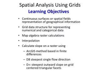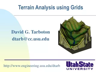
Spatial Analysis Using Grids
Spatial Analysis Using Grids . Learning Objectives. The concepts of spatial fields as a way to represent geographical information Raster and vector representations of spatial fields Perform raster calculations using spatial analyst Raster calculation concepts and their use in hydrology

Spatial Analysis Using Grids
E N D
Presentation Transcript
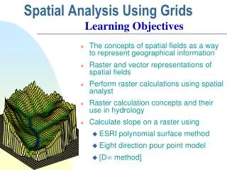
Spatial Analysis Using Grids Learning Objectives • The concepts of spatial fields as a way to represent geographical information • Raster and vector representations of spatial fields • Perform raster calculations using spatial analyst • Raster calculation concepts and their use in hydrology • Calculate slope on a raster using • ESRI polynomial surface method • Eight direction pour point model • [D method]
Readings – at http://help.arcgis.com • Elements of geographic information starting from “Overview of geographic information elements” http://help.arcgis.com/en/arcgisdesktop/10.0/help/00v2/00v200000003000000.htm to “Example: Representing surfaces”
Readings – at http://help.arcgis.com • Rasters and images starting from “What is raster data” http://help.arcgis.com/en/arcgisdesktop/10.0/help/index.html#//009t00000002000000.htm to end of “Raster dataset attribute tables”
(x1,y1) y f(x,y) x Two fundamental ways of representing geography are discrete objects and fields. The discrete object view represents the real world as objects with well defined boundaries in empty space. Points Lines Polygons The field view represents the real world as a finite number of variables, each one defined at each possible position. Continuous surface
Raster and Vector Data Raster data are described by a cell grid, one value per cell Vector Raster Point Line Zone of cells Polygon
Raster and Vector are two methods of representing geographic data in GIS • Both represent different ways toencode andgeneralizegeographic phenomena • Both can be used to code both fields and discrete objects • In practice a strong association between raster and fields and vector and discrete objects
Numerical representation of a spatial surface (field) Grid TIN Contour and flowline
Six approximate representations of a field used in GIS Regularly spaced sample points Irregularly spaced sample points Rectangular Cells Irregularly shaped polygons Triangulated Irregular Network (TIN) Polylines/Contours from Longley, P. A., M. F. Goodchild, D. J. Maguire and D. W. Rind, (2001), Geographic Information Systems and Science, Wiley, 454 p.
A grid defines geographic space as a matrix of identically-sized square cells. Each cell holds a numeric value that measures a geographic attribute (like elevation) for that unit of space.
The grid data structure • Grid size is defined by extent, spacing and no data value information • Number of rows, number of column • Cell sizes (X and Y) • Top, left , bottom and right coordinates • Grid values • Real (floating decimal point) • Integer (may have associated attribute table)
Definition of a Grid Cell size Number of rows NODATA cell (X,Y) Number of Columns
Floating Point Grids Continuous data surfaces using floating point or decimal numbers
Value attribute table for categorical (integer) grid data Attributes of grid zones
Raster Sampling from Michael F. Goodchild. (1997) Rasters, NCGIA Core Curriculum in GIScience, http://www.ncgia.ucsb.edu/giscc/units/u055/u055.html, posted October 23, 1997
Raster Generalization Largest share rule Central point rule
Raster Calculator Example 5 6 Precipitation - Losses (Evaporation, Infiltration) = Runoff 7 6 Cell by cell evaluation of mathematical functions - 3 3 2 4 = 2 3 5 2
Runoff generation processes P Infiltration excess overland flow aka Horton overland flow f P qo P f Partial area infiltration excess overland flow P P qo P f P Saturation excess overland flow P qo P qr qs
Runoff generation at a point depends on • Rainfall intensity or amount • Antecedent conditions • Soils and vegetation • Depth to water table (topography) • Time scale of interest These vary spatially which suggests a spatial geographic approach to runoff estimation
Cell based discharge mapping flow accumulation of generated runoff Radar Precipitation grid Soil and land use grid Runoff grid from raster calculator operations implementing runoff generation formula’s Accumulation of runoff within watersheds
Raster calculation – some subtleties Resampling or interpolation (and reprojection) of inputs to target extent, cell size, and projection within region defined by analysis mask + = Analysis mask Analysis cell size Analysis extent
40 50 55 42 47 43 42 44 41 Spatial Snowmelt Raster Calculation Example 100 m 150 m 100 m 150 m 4 6 2 4
New depth calculation using Raster Calculator “snow100” - 0.5 * “temp150”
The Result • Outputs are on 150 m grid. • How were values obtained ? 38 52 41 39
100 m 40 50 55 42 47 43 150 m 6 4 42 44 41 2 4 Nearest Neighbor Resampling with Cellsize Maximum of Inputs 40-0.5*4 = 38 55-0.5*6 = 52 38 52 42-0.5*2 = 41 41-0.5*4 = 39 41 39
Scale issues in interpretation of measurements and modeling results The scale triplet a) Extent b) Spacing c) Support From: Blöschl, G., (1996), Scale and Scaling in Hydrology, Habilitationsschrift, Weiner Mitteilungen Wasser Abwasser Gewasser, Wien, 346 p.
From: Blöschl, G., (1996), Scale and Scaling in Hydrology, Habilitationsschrift, Weiner Mitteilungen Wasser Abwasser Gewasser, Wien, 346 p.
Use Environment Settings to control the scale of the output Extent Spacing & Support
Raster Calculator “Evaluation” of “temp150” 4 6 6 6 4 4 4 2 4 2 2 4 4 Nearest neighbor to the E and S has been resampled to obtain a 100 m temperature grid.
47 52 38 41 45 41 41 39 42 Calculation with cell size set to 100 m grid “snow100” - 0.5 * “temp150” • Outputs are on 100 m grid as desired. • How were these values obtained ?
100 m 40 50 55 42 47 43 42 44 41 100 m cell size raster calculation 40-0.5*4 = 38 50-0.5*6 = 47 55-0.5*6 = 52 42-0.5*2 = 41 38 47 52 47-0.5*4 = 45 43-0.5*4 = 41 41 45 41 42-0.5*2 = 41 44-0.5*4 = 42 6 6 4 39 150 m 42 41 6 4 41-0.5*4 = 39 2 4 4 Nearest neighbor values resampled to 100 m grid used in raster calculation 2 4 2 4 4
What did we learn? • Raster calculator automatically uses nearest neighbor resampling • The scale (extent and cell size) can be set under options • What if we want to use some other form of interpolation? • From Point • Natural Neighbor, IDW, Kriging, Spline, … • From Raster • Project Raster (Nearest, Bilinear, Cubic)
Interpolation Estimate values between known values. A set of spatial analyst functions that predict values for a surface from a limited number of sample points creating a continuous raster. Apparent improvement in resolution may not be justified
Interpolation methods • Nearest neighbor • Inverse distance weight • Bilinear interpolation • Kriging (best linear unbiased estimator) • Spline
Spline Interpolation Nearest Neighbor “Thiessen” Polygon Interpolation
Interpolation Comparison Grayson, R. and G. Blöschl, ed. (2000)
Further Reading Grayson, R. and G. Blöschl, ed. (2000), Spatial Patterns in Catchment Hydrology: Observations and Modelling, Cambridge University Press, Cambridge, 432 p. Chapter 2. Spatial Observations and Interpolation Full text online at: http://www.catchment.crc.org.au/special_publications1.html
Spatial Surfaces used in Hydrology Elevation Surface — the ground surface elevation at each point
3-D detail of the Tongue river at the WY/Mont border from LIDAR. Roberto Gutierrez University of Texas at Austin
Topographic Slope • Defined or represented by one of the following • Surface derivative z (dz/dx, dz/dy) • Vector with x and y components (Sx, Sy) • Vector with magnitude (slope) and direction (aspect) (S, )
a b c d e f g h i ArcGIS “Slope” tool
Example a b c 30 d e f 145.2o 80 74 63 69 67 56 g h i 60 52 48
80 80 74 74 63 63 69 69 67 67 56 56 60 60 52 52 48 48 Hydrologic Slope (Flow Direction Tool) - Direction of Steepest Descent 30 30 Slope: