Spatial Econometric Analysis Using GAUSS
Spatial Econometric Analysis Using GAUSS. 2 Kuan-Pin Lin Portland State University. GAUSS Mathematical and Statistical System. Windows Interface Windows Command, Error, Log, … Menu File, Edit, Run, …, Help Operation Interactive Mode Command (Input / Output) Batch Mode Writing Program


Spatial Econometric Analysis Using GAUSS
E N D
Presentation Transcript
Spatial Econometric AnalysisUsing GAUSS 2 Kuan-Pin LinPortland State University
GAUSSMathematical and Statistical System • Windows Interface • Windows • Command, Error, Log, … • Menu • File, Edit, Run, …, Help • Operation • Interactive Mode • Command (Input / Output) • Batch Mode • Writing Program • Online Help
GAUSS Basics • Basic Operations on Matrices + - ^ .* ./ % ! * / .< .<= .== .>= .> ./= < <= == >= > /= .not .and .or .xor not and or xor ~ | .*. *~ • Special Operators [] {} : . '(transpose) • Useful Algrbra and Matrix Operations exp ln log abs sqrt pi sin cos inv invpd(inverse) det(determinant) • Example • Least Squares: b=y/x
GAUSS ProgrammingUseful GAUSS Functions • System Functions: use, load, output • Data Generating Functions:ones, zeros, eye, seqa, seqm, rndu, rndn • Data Conversion Functions:reshape, selif, delif, vec, vech, xpnd, submat, diag, diagrv • Basic Matrix Functions: • Matrix Description:rows, cols, maxc, minc, meanc, median, stdc • Matrix Operations:sumc,cumsumc,prodc,cumprodc,sortc,sorthc,sortind • Matrix Computation:det,inv,invpd,solpd,vcx,corrx,cond,rank,eig,eigh • Probability and Statistical Functions:pdfn, cdfn, cdftc, cdffc, cdfchic, dstat, ols • Calculus Functions:gradp, hessp, intsimp, linsolve, eqsolve, sqpsolve
GAUSS ProgrammingControlling Execution Flow • If Statementif; then; else; elseif; endif; • For Loopfor i (start,stop,step); ... endfor; • Do Loopdo while ... endo;do until ... endo;
GAUSS ProgrammingWrite Your Own Functions • Single Line Functionfn fn_name(args) = code_for_function; • Procedureproc [[(nrets)=]] proc_name(arg_list);local list of local variables;... statements in the body of procedure;retp(ret_list);endp;
GAUSS ProgrammingExample 1 • Do you know the accuracy of your computer's numerical calculation? This example addresses this important problem. Suppose e is a known small positive number, and the 5x4 matrix X is defined as follows: Verify that the eigenvalues of X'X are 4+e2, e2, e2, and e2. How small of the value of e your computer will allow so that X'X can be inverted? (example.1)
GAUSS ProgrammingExample 2 • Write a single-line GAUSS function to convert a quarterly time series into the annual series by taking the average of every four data points. How you extend the single-line version of time series conversion function to a multi-line procedure so that it can handle the conversion of more than one time series? (example.2)
GPE2 for GAUSS • GPE2 is a package of econometric procedures written in GAUSS. There are four main functions, driven by a set of global control variables: • ResetSet up global control (input and output) variables. • EstimateEstimation of a linear or generalized linear model. • ForecastForecasting based on a linear or generalized linear model. • OptimizeEstimation of a nonlinear model. • GpehelpOnline help of using GPE2.
GPE2 for GAUSSSelected Global Control Variables • Input Control Variables_names, _begin, _end, _rstat, _rtest, _rplot, _rlist,_const, _restr, _vcov, _hacv, _weight, _ivar, _dlags, _pdl, _eq, _id, _ar, _ma, _arma, _garch, _acf, _acf2, _nlopt, _method, _iter, _tol, _step, _conv, _fbrgin, _fend, _fstat, _fplot, _splag, _spw, _spwd • Output Control Variables__y, __x, __e, __b, __vb, __v, __rss, __r2, __f, __vf, __t, __a, __va
GPE2 for GAUSSA Typical Program Using GPE2 • /* • ** Comments on program title, purposes, and the usage of the program • */ • use gpe2; @ using GPE package (version 2) @ • // this must be the first executable statement • /* • ** Writing output to file or sending it to printer: • ** specify file name for output • */ • // Loading data: read data series from data files. • /* • ** Generating or transforming data series: • ** create and generate variables with data scaling or transformation • ** (e.g. y and x are generated here and will be used below) • */ • call reset; @ initialize global variables @ • /* • ** Set input control variables for model estimation • ** (e.g. _names for variable names, see Appendix A) • */ • call estimate(y,x); @ do model estimation @ • // variables y, x are generated earlier • /* • ** Retrieve output control variables for model evaluation and analysis • */ • /* • ** Set more input control variables if needed, for model prediction • ** (e.g. _b for estimated parameters) • */ • call forecast(y,x); @ do model prediction @ • end; @ important: don’t forget this @
GPE2 for GAUSSExamples • More than 70 examples covering linear and nonlinear least squares, instrumental variables, system of simultaneous linear equations, time series analysis, panel data, limited dependent variables, maximum likelihood, generalized methods of moments, and … • The latest extensions include spatial lag model estimation, hypothesis testing, and robust inference.
Software Demonstration • Installation • GAUSS Light 10.0 • GPE2 for GAUSS 10.0 • Example: Zellner and Revankar [1970]U.S. Transportation Equipment Industry • Cobb-Douglas Production Functionln(Q) = a + b ln(L) + g ln(K) + e • Generalized Cobb-Douglas Production Functionln(Q) + q Q = a + b ln(L) + g ln(K) + e
ExampleZellner and Revankar [1970] • Cobb-Douglas Production Function • OLS Estimator • Hypothesis Testing • Constant Returns to Scale? • Homoscedasticity? • Generalized Production Function • Output Effects? • Instrumental Variables • GAUSS/GPE2 Program and Data
References • K.-P. Lin, Computational Econometrics: GAUSS Programming for Econometricians and Financial Analysts, ETEXT Publishing, Los Angeles, 2001. • C.-F. Chung, Learning Econometrics with GAUSS, Institute of Economics, Academia Sinica, 2000. • A. Zellner and N. Revankar, "Generalized Production Functions," Review of Economic Studies, 1970, 241-250.