Two Example Ground Water Mounding Situations
Two Example Ground Water Mounding Situations. John L. Nieber Department of Biosystems and Agricultural Engineering University of Minnesota. Ground Water Mounding Beneath a Stormwater Basin. Study conducted in Washington Co. by Emmons & Olivier Associates

Two Example Ground Water Mounding Situations
E N D
Presentation Transcript
Two Example Ground Water Mounding Situations John L. Nieber Department of Biosystems and Agricultural Engineering University of Minnesota
Ground Water Mounding Beneath a Stormwater Basin • Study conducted in Washington Co. by Emmons & Olivier Associates • Results presented here are from a report to the MPCA and also from the M.S. thesis (May 2005) of Jennifer Olson.
CD-P85 • Natural infiltration basin • 30 acres in extent • 29 feet deep • Outwash material • 7 wells • Pump station links CD-P85 with City stormwater system
Water levels in monitoring wells near CD-P85 Note the two scales for water levels
Models Used for Simulations • Hantush mounding model – simple analytical model, most common ground water mounding equation • Multi Layer Analytic Element Model (MLAEM) – has been used at this site in past, regional flow model in TCMA • FEMWATER – unsaturated/saturated flow model, recommended in literature for complex systems
Model Input • Identical parameters used when applicable • Measured parameters • Recharge area, recharge rate, duration (transient vs. steady state models), depth to water table, saturated thickness, initial ground water elevation, bedrock elevation, nearby lake elevations • Literature value (unknown) parameters • Saturated hydraulic conductivity (calibrated model, slug test) • Porosity (effective and fillable) • Unsaturated flow characteristics • Used first dataset (July 2002) to determine unknown parameters
Model Selection • Sum of square differences • MLAEM model – closest to observed values • Unable to calibrate porosity and Ksat to desired accuracy – steady state • Hantush model – second best • Calibration parameters include Ksat and porosity – most variable and unknown parameters
Some WSAS Mounding Effects Analysis performed with COMSOL MP3.2 Finite Element Solution of the Richards Equation
Vertical section showing five leach trenches and a perching layer
120 gallons/day/foot; Ks = 2.8 feet/day Kperch layer = 0.28 feet/day
120 gallons/day/foot; Ks = 2.8 feet/day Kperch layer = 0.28 feet/day
18 gallons/day/foot; Ks = 2.8 feet/day Kperch layer = 0.028 feet/day
7 gallons/day/foot; Ks = 2.8 feet/day Kperch layer = 0.0028 feet/day
246 gallons/day/foot; Ks = 2.8 feet/day Kperch layer = 2.8 feet/day
175 gallons/day/foot; Ks = 2.8 feet/day Kellipses = 0.28 feet/day
Summary Low perm layers do not need to be continuous to affect septic infiltration rate