Understanding the Two Tank System: Op-Amp Circuit Models and Transformations
This document explores the two tank system in electrical engineering, focusing on an operational amplifier circuit example. It discusses the relationships between input and output voltages, KCL analysis, and the application of transfer function and state-space models. By detailing the steps for transforming state-space models into transfer functions using Laplace transforms, it provides practical examples using MATLAB code. Illustrates how to derive system dynamics, enabling better understanding of I/O models, linear systems, and the integration of mechanical and electromechanical elements.

Understanding the Two Tank System: Op-Amp Circuit Models and Transformations
E N D
Presentation Transcript
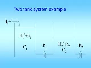
In eq pt: all flow=same 1 3 2 4
Op Amp circuit example Note: ip1=0, ∴vp1=vo=vA & vB=vp2=0 Let vC1 & vC2 be s.v., vo output.
KCL at A: vo is not s.v. nor input, use vo=vC2
KCL at B: 0 vo1 not s.v. nor input, vo1=vA+vC1=vn1+vC1 =vp1+vC1=vo+vC1 =vC2+vC1
Modeling • Types of systems electric mechanical electromechanical • Types of models I/O o.d.e. models Transfer Function state space models
I/O o.d.e. model: a d.e. involving input/output only. linear: where u: input y: output
State space model: linear: or in some text: where: u: input y: output x: state vector A,B,C,D, or F,G,H,J are const matrices
Other types of models: Transfer function model (This is I/O model) from I/O o.d.e. model, take Laplace transform:
Then I/O model in L.T. domain becomes: This is the T.F. model of the system. ∴T.F. or i.e. output L.T. is eq. to input L.T. with gain H(s) denote
State space model to T.F. / block diagram: s.s. Take L.T. : From sX(s)-AX(s)=BU(s) sIX(s)-AX(s)=BU(s) (sI-A)X(s)=BU(s) X(s)=(sI-A)-1BU(s) 1 2 1
2 into : Y(s)=C(sI-A)-1BU(s)+DU(s) Y(s)=[C(sI-A)-1B+D] U(s) H(s)= D+C(sI-A)-1B is the T.F. from u to y from 1
>> n=[1 2 3];d=[1 4 5 6]; >> [A,B,C,D]=tf2ss(n,d) A = -4 -5 -6 1 0 0 0 1 0 B = 1 0 0 C = 1 2 3 D = 0 >> tf(n,d) Transfer function: s^2 + 2 s + 3 --------------------- s^3 + 4 s^2 + 5 s + 6 • In Matlab: >> A=[0 1;-2 -3]; >> B=[0;1]; >> C=[1 3]; >> D=[0]; >> [n,d]=ss2tf(A,B,C,D) n = 0 3.0000 1.0000 d = 1 3 2