Mapping the AES Algorithm to MorphoSys Architecture
This document provides a comprehensive overview of the AES (Advanced Encryption Standard) algorithm, including its introduction, development timeline, and mapping to the MorphoSys architecture for performance evaluation. It outlines the basic structure of AES encryption and decryption, detailing the key expansion, data processing steps, and the mathematical background involved, such as Galois Field operations. By demonstrating how AES can be effectively implemented in MorphoSys, the paper highlights both its security capabilities and performance benefits in hardware and software environments.


Mapping the AES Algorithm to MorphoSys Architecture
E N D
Presentation Transcript
Mapping the AES Algorithmto MorphoSys Architecture Ye Tang Aug 2001
Overview • Part I: AES Algorithm Introduction • Part II: Mapping to MorphoSys • Part III: Performance Evaluation
What Is AES? • Advanced Encryption Standard • Next generation cryptographic algorithm for use by U.S. Government organizations to protect sensitive (unclassified) information. • Will hopefully replace the current standard, DES (Data Encryption Standard) and Triple DES, sooner or later.
AES Development Timeline • National Institute of Standards and Technology (NIST) worked with the whole industry and the cryptographic community to develop AES • Jan 1997: NIST announced the initiation of the AES development • Aug 1998: NIST announced that fifteen algorithms were selected as candidates • Apr 1999: NIST selected five algorithms from the fifteen as the AES finalist • Oct 2000: NIST announced that Rijndael has been selected for the AES. • Feb 2001: Draft FIPS for the AES published for public comments. • May 2001: Comment period closes. • ? 2001: AES FIPS becomes official.
Rijndael Overview • A symmetric block cipher developed by two Belgium cryptology experts, Joan Daemen and Vincent Rijmen • Apply to data blocks of 128 bits, using cipher keys with lengths of 128, 192, and 256 bits • Very good performance in both hardware and software across a wide range of computing • Very high security level. Even with future advances in technology, it has the potential to remain secure well beyond twenty years.
Terms Used in Rijndael • Round • Rijndael is an iterated block cipher. Every iteration is called Round. Rijndael has 10, 12, or 14 Rounds when the Cipher Key size is 128, 192, or 256 bits, respectively. • Cipher Key • Original secret key used for encryption or decryption. Also shortened as “Key”. The size can be 128, 192, or 256 bits. • Round Key • A series of keys derived from the Cipher Key. Every Round needs a Round Key, Round Key’s size can only be 128 bits. • Key Expansion • the routine used to generate all Round Keys from the Cipher Key.
Basic Structure of Encryption • Initialization • Key Expansion: Get all necessary Round Keys from the Cipher Key. • Data Processing • Initial step • RoundKeyAddition() • Intermediate Rounds (10, 12, or 14 Rounds) • SubBytes() • ShiftRows() • MixColumns() • RoundKeyAddition() • Final Round • SubBytes() • ShiftRows() • RoundKeyAddition() A BSMA BSMA … BSA
Basic Structure of Decryption • Initialization • Key Expansion: Get all necessary Round Keys from the Cipher Key. The detailed procedure is different than Encryption’s. • Data Processing (Replace with inverse functions) • Initial step • InvRoundKeyAddition() • Intermediate Rounds (10, 12, or 14 Rounds) • InvSubBytes() • InvShiftRows() • InvMixColumns() • InvRoundKeyAddition() • Final Round • InvSubBytes() • InvShiftRows() • InvRoundKeyAddition() same sequence:A BSMA BSMA … BSA
Math Background (1) • Galois Field GF(28) • A byte b, consisting of bits b7 b6 b5 b4 b3 b2 b1 b0 is considered as a polynomial with coefficient in {0,1}: b7x7 + b6x6 + b5x5 + b4x4 + b3x3 + b2x2 + b1x1 + b0 • Addition • Coefficients are given by the sum of the coefficients of the two terms modulo 2 Example: ’57’+’83’=‘D4’ (hexadecimal) (x6 + x4 + x2 + x + 1) + (x7 + x +1) = x7 + x6 + x4 + x2 • Addition corresponds with bitwise XOR: ’57’ ’83’=‘D4’ • Subtraction (i.e., inverse of addition) • the same as addition (also bitwise XOR)
Math Background (2) • Multiplication • Multiplication in GF(28) corresponds with multiplication of polynomials modulo an irreducible binary polynomial of degree 8. For Rijndael, this irreducible polynomial is called m(x) and given by m(x) = x8 + x4 + x3 + x + 1 Example: ’57’ ’83’=‘C1’ (x6 + x4 + x2 + x + 1)(x7 + x +1) = x13 + x11 + x9 + x8 +x7 +x7 + x5 + x3 + x2 + x + x6 + x4 + x2 + x +1 = x13 + x11 + x9 + x8 +x6 + x5 + x4 + x3 + 1 x13 + x11 + x9 + x8 +x6 + x5 + x4 + x3 + 1 modulo x8 + x4 + x3 + x + 1 = x7 + x6 + 1 result
Math Background (3) • Multiplication by x (xtime operation) • result before modulo m(x) is: b7x8 + b6x7 + b5x6 + b4x5 + b3x4 + b2x3 + b1x2 + b0x • If b7 = 0, no reduction; • If b7 = 1, m(x) must be subtracted (i.e., XORed) • In other words, b(x) * x can be implemented as a one-bit left shift and a subsequent conditional XOR with ‘1B’. • Multiplication by x is denoted by a = xtime(b) • Example: ’57’ * ’02’ = xtime(’57’) = (0)10101110 = ‘AE’’57’ * ’04’ = xtime(xtime(‘57’)) = xtime(‘AE’) = (1)01011100 ^ ‘1B’ = ’47’
Math Background (4) • How to do multiplication in Rijndael? (e.g. ’57’ * ’13’) • 1st Approach: use table-lookup (two tables: Log & Alog) mul(’57’,’13’) = Alogtable[(Logtable[’57’]+Logtable[’13’])%255]= Alogtable[(98+14)%255] = Alogtable[112] = 254 = ‘FE’ • logarithmic table and anti-logarithmic table are used • 2nd Approach: use xtime operation ’57’ * ’13’ = ’57’ * (’01’ ^ ’02’ ^ ’10’) = ’57’ * ’01’ ^ ’57’ * ’02’ ^ ’57’ * ’10’ = ’57’ ^ ‘AE’ ^ ’07’ = ‘FE’ Notice:xtime can be implemented directly by hardware. But in MorphoSys, it is still implemented by table lookup. The difference with the 1st approach is it needs only one table.
Math Background (5) • Polynomial multiplication a(x) = a3x3 + a2x2 + a1x1 + a0 b(x) = b3x3 + b2x2 + b1x1 + b0 c(x) = a(x) * b(x) = (c6x6 + c5x5 + c4x4 + c3x3 + c2x2 + c1x1 + c0) d(x) = c(x) mod (x4 + 1) Final Result After some simplification, d(x) can be represented as:
Basic Function 1a: SubBytes() • ‘b’ = SubBytes(‘a’) • Substitute ‘a’ with ‘b’ which is the element at address ‘a’ in table S-box. • table S-box is a predefined 256-byte constant table. • Example: SubBytes(’00’) = ’63’ (’63’ is the first element in S-box)
Basic Function 1b: InvSubBytes() • Similar to SubBytes() • Only difference: the table is “Inv S-box”, another predefined 256-byte constant table.
Basic Function 2a: ShiftRows() • Each row is shifted over different offsets: Row 0, 1, 2, 3 will be shifted over 0, 1, 2, 3 byte(s), respectively. The number represents the position of the corresponding byte
Basic Function 2b: InvShiftRows() • Similar to ShiftRows() • Row 0, 1, 2, 3 will be shifted over 0, 3, 2, 1 byte(s), respectively. Notice the positions are restored to original ones if InvShiftRows() is applied after ShiftRows()
Basic Function 3a: MixColumns() • The following polynomial multiplication is performed for every column: where c(x) = ’03’x3 + ’01’x2 + ’01’x + ’02’ i.e.,
Basic Function 3b: InvMixColumns() • Similar to MixColumns() • Uses c-1(x) instead of c(x) c-1(x) = ’0B’x3 + ’0D’x2 + ’09’x + ’0E’
xtime Approach for MixColumns()… d0 = ’02’*a0 + ’03’*a1 + ’01’ *a2 + ’01’ *a3 = a0 + (a0 + a1 + a2 + a3) + ’02’*(a0 + a1) 1st element notice a0 + a0 = 0 (XOR) tmp = a0 ^ a1 ^ a2 ^ a3; tm = a0 ^ a1; tm = xtime(tm); a0 ^ = tm ^ tmp; tm = a1 ^ a2; tm = xtime(tm); a1 ^ = tm ^ tmp; tm = a2 ^ a3; tm = xtime(tm); a2 ^ = tm ^ tmp; tm = a3 ^ a0; tm = xtime(tm); a3 ^ = tm ^ tmp;
… and InvMixColumns() d(x) = c-1(x) * a(x) where c-1(x) = ’0B’x3 + ’0D’x2 + ’09’x + ’0E’ d0 = ’0E’*a0 + ’0B’*a1 + ’0D’*a2 + ’09’*a3 = a0 + (a0 + a1 + a2 + a3) + ’02’*(a0 + a1) + ’04’*(a0 + a2) + ’08’*(a0 + a1 + a2 + a3) more xtime operations tmp1 = a0 ^ a1 ^ a2 ^ a3; tmp2=xtime(xtime(xtime(tmp1))); tm1 = a0 ^ a2; tm2 = a0 ^ a1; tm1 = xtime(xtime(tm1)); tm2 = xtime(tm2); a0 ^ = tm1 ^ tm2 ^ tmp1 ^ tmp2; tm1 = a1 ^ a3; tm2 = a1 ^ a2; tm1 = xtime(xtime(tm1)); tm2 = xtime(tm2); a1 ^ = tm1 ^ tm2 ^ tmp1 ^ tmp2; tm1 = a2 ^ a0; tm2 = a2 ^ a3; tm1 = xtime(xtime(tm1)); tm2 = xtime(tm2); a2 ^ = tm1 ^ tm2 ^ tmp1 ^ tmp2; tm1 = a3 ^ a1; tm2 = a3 ^ a0; tm1 = xtime(xtime(tm1)); tm2 = xtime(tm2); a3 ^ = tm1 ^ tm2 ^ tmp1 ^ tmp2;
Basic Function 4a: AddRoundKey() • A 16-byte Round Key is added (i.e., bitwise XORed) to the 16-byte data block. Each data byte is added with the same position Round Key byte.
Basic Function 4b: InvAddRoundKey() • Exactly the same as AddRoundKey() • This is because subtraction is the same as addition
Key Expansion for Encryption • Key Expansion is the process of generating Round Keys from the Cipher Key. Length of Round Keys = Block Length * (Number of Rounds +1) e.g., If key size is 128 bits, 10 Rounds are needed, thus 128 * 11 = 1408 bits are needed for Round keys. • Need table lookup operation • tables needed: • S-box: 256 bytes • Rcon: 30 bytes • Pseudo Code: next slide
Pseudo Code for Key Expansion KeyExpansion (Key[4*Nk], W[4*(Nr+1)], Nk) { for ( i = 0; i < Nk; i++) W[i] = (Key[4*i], Key[4*i+1], Key[4*i+2], Key[4*i+3]); for ( i = Nk; i < 4*(Nr+1); i++) { temp = W[i-1]; if ( i % Nk == 0) temp = SubWord(RotWord(temp)) ^ Rcon[i/Nk]; else if ( Nk = 8 and i % Nk == 4) temp = SubWord(temp); W[i] = W[i-Nk] ^ temp; } } SubWord (W(a, b, c, d)) { return W(S-box(a), S-box(b), S-box(c), S-box(d)); } RotWord (W(a, b, c, d)) {return W(b, c, d, a); }
Key Expansion for Decryption • First, apply the same expansion procedure as in Encryption. • Second, apply InvMixColumns() to every Round Key except the first and last one. • There are (# of Rounds+1) Round Keys in total. So (# of Rounds-1) Round Keys will be applied to InvMixColumns(). • Tables needed: • S-box: 256 bytes • Rcon: 30 bytes • Log: 256 bytes • Alog: 256 bytes • for InvMixColumns(), do not use xtime approach here because Key Expansion is done by TinyRISC and there is enough memory to save tables
Important upgrades in M2 • M2 is the next generation MorphoSys architecture • Some new features important to AES implementation • Every RC can do table lookup operation locally. This is realized by an embedded 512-byte memory in each RC. • The number of registers in each RC is increased from 4 to 8.
Key Expansion Implementation • Completely done by the general-purpose RISC processor in MorphoSys: TinyRISC • The resulted Round Keys are saved in main (external) memory for future use
Issues in Data Processing Part • RC Array Partition • How to Do (Inv)ShiftRows() • About (Inv)MixColumns()
Issue 1: RC Array Partition • Compute in parallel • 4 data blocks, or 64 bytes, are processed at the same time by 64 RCs • RC Array partition: choose the scenario on the right. • though not intuitive, it provides natural data loading/storing order. • Thanks to the efficient interconnection network in MorphoSys, the subsequent data move is still kept simple. good! 8x8 8x8
Issue 2: How to Do (Inv)ShiftRows()? • In intermediate Rounds, (Inv)ShiftRows() is only a position adjustment for the subsequent (Inv)MixColumns(). • It is desirable to have every RC save the data needed for (Inv)MixColumns, i.e., the data in the same column, during (Inv)ShiftRows(). This will make (Inv)MixColumns() faster. • But in the final round, no (Inv)MixColumns() follows ShiftRows(). So a simpler data move strategy is used there.
Data Move for ShiftRows()in intermediate Rounds • Eight steps are needed. The goal is shown below: only one block is shown here order is not important
Intermediate ShiftRows(): Step 1 Express Lane, Row mode means rk in Rowi
Intermediate ShiftRows(): Step 2 Express Lane, Row mode means rk in Rowi
Intermediate ShiftRows(): Step 3, 4 Mux A = Left (r), Column mode means rk in Columni all seeds are ready
Intermediate ShiftRows(): Step 5 Express Lane, Row mode means rk in Rowi seeds
Intermediate ShiftRows(): Step 6 Express Lane, Row mode means rk in Rowi
Intermediate ShiftRows(): Step 7 Express Lane, Row mode means rk in Rowi
Intermediate ShiftRows(): Step 8 Express Lane, Row mode means rk in Rowi
Data Move for InvShiftRows()in intermediate Rounds • Similarly, eight steps are needed. The goal is: only one block is shown here order is not important
Intermediate InvShiftRows(): Step 1 Express Lane, Row mode means rk in Rowi
Intermediate InvShiftRows(): Step 2 Express Lane, Row mode means rk in Rowi
Intermediate InvShiftRows(): Step 3, 4 Mux A = Left (r), Column mode means rk in Columni all seeds are ready
Intermediate InvShiftRows(): Step 5 Express Lane, Row mode means rk in Rowi seeds
Intermediate InvShiftRows(): Step 6 Express Lane, Row mode means rk in Rowi
Intermediate InvShiftRows(): Step 7 Express Lane, Row mode means rk in Rowi
Intermediate InvShiftRows(): Step 8 Express Lane, Row mode means rk in Rowi
Data Move for ShiftRows()in Final Round • Five steps are needed. The goal is: only one block is shown here only use r0 for result