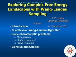
Wang-Landau Sampling in Statistical Physics
FSU National Magnet Lab Winter School Jan. 12, 2012. D P Landau Center for Simulational Physics The University of Georgia. Wang-Landau Sampling in Statistical Physics. Introduction Basic Method Simple Applications (how well does it work?) 2 nd order transitions – 2d Ising model

Wang-Landau Sampling in Statistical Physics
E N D
Presentation Transcript
FSU National Magnet Lab Winter School Jan. 12, 2012 D P LandauCenter for Simulational PhysicsThe University of Georgia Wang-Landau Sampling in Statistical Physics • Introduction • Basic Method • Simple Applications (how well does it work?) • 2nd order transitions – 2d Ising model • 1st Order transition – 2d Potts Models • Critical endpoint - triangularIsing model • Some Extensions • Conclusions
Introductory Comments An understanding of materials behavior at non-zero temperature cannot be obtained solely from knowledge of T=0 properties. For this we need to use statistical mechanics/thermodynamics coupled with “knowledge” of the interatomic couplings and interactions with any external fields. This can be a very difficult problem!
Simulation NATURE Experiment Theory
Reminder from Statistical Mechanics ThePartition functioncontains all thermodynamic information: The probability of the nth state appearing is: Thermodynamic properties are then determined from the free energy Fwhere F=-kBTlnZ
Reminder from Statistical Mechanics ThePartition functioncontains all thermodynamic information: Metropolis Monte Carlo approach: sample states via a random walk in probability space The “fruit fly” of statistical physics: The Ising model For a system of N spins have 2N states!
Single Spin-Flip Monte Carlo Method Typical spin configurations for the Ising square lattice with pbc T << Tc T~Tc T>>Tc
Single spin-flip sampling for the Ising model Produce the nth state from the mth state … relative probability is Pn/Pm need only the energy difference,i.e. E=(En-Em)between the states Any transition rate that satisfiesdetailed balanceisacceptable, usually the Metropolis form(Metropolis et al, 1953).W(mn) = o-1exp (-E/kBT), E > 0= o-1 , E < 0 where o is the time required to attempt a spin-flip.
Metropolis Recipe: 1. Choose an initial state 2. Choose a sitei 3. Calculate the energy changeEthat results if the spin at siteiis overturned 4. Generate a random numberrsuch that0 < r < 1 5.If r < exp(-E/kBT), flip the spin 6. Go to 2. This is not a unique solution. An alternative(Glauber, 1963): Wnm=o-1[1+itanh (Ei /kBT)], where iEi is the energy of the ith spin in state n. Both Glauber and Metropolis algorithms are special cases of a general transition rate(Müller-Krumbhaar and Binder, 1973)
Correlation times Define an equilibrium relaxation function(t) and i.e. diverges at Tc!
Problems and Challenges Statics:Monte Carlo methods are valuable, but near Tc critical slowing downfor2nd ordertransitions metastabilityfor1st ordertransitions Try to reduce characteristic time scales or circumvent them “Dynamics”:stochastic vs deterministic
Multicanonical Sampling The canonical probabilityP(E)may contain multiple maxima, widely spaced in configuration space (e.g. 1st order phase transition, etc.) Standard methods become “trapped” near one maximum; infrequent transitions between maxima leads to poor relative weights of the maxima and the minima of P(E). modify the single spin flip probability to enhance the probability of the “unlikely” states between the maxima accelerates effective sampling! Reformulate the problem an effective Hamiltonian Berg and Neuhaus (1991)
Compare ensembles: Then, Thermodynamic variable
Compare ensembles: But, finding Heff isn’t easy Then, Thermodynamic variable
Parallel tempering (replica exchange) Create multiple systems at differentTi T1 T2 T3 T4 T5 . . . Define i = 1/Ti Hukushima and Nemoto (1996); Swendsen and Wang (1986)
Parallel tempering (replica exchange) Create multiple systems at differentTi T1 T2 T3 T4 T5 . . . Define i = 1/Ti Simulate all systems simultaneously Hukushima and Nemoto (1996); Swendsen and Wang (1986)
Parallel tempering (replica exchange) Create multiple systems at differentTi T1 T2 T3 T4 T5 . . . Define i = 1/Ti Simulate all systems simultaneously At regular intervals interchange configurations at neighboring T with probability P given by: Energy of state i
Parallel tempering (replica exchange) Create multiple systems at differentTi T1 T2 T3 T4 T5 . . . Define i = 1/Ti But, the Ti must be chosen carefully Simulate all systems simultaneously At regular intervals interchange configurations at neighboring T with probability P given by: Energy of state i
Types of Computer Simulations Deterministic methods . . . (Molecular dynamics) Stochastic methods . . . (Monte Carlo)
Improvements in Performance (Ising model): Computer speed Algorithmic advances - cluster flipping, reweighting. . . 1E10 1E9 1E8 relative performance 1E7 1000000 100000 10000 1000 100 computer speed 10 1 1970 1975 1980 1985 1990 1995 2000
The “Random Walk in Energy Space with a Flat Histogram” method or “Wang-Landau sampling”
A Quite Different Approach Random Walk in Energy Space with a Flat HistogramReminder: Estimate the density of statesg(E) directly –– how?1.Set g(E)=1; choose a modification factor(e.g. f0=e1) 2. Randomly flip a spin with probability: 3.Setg(Ei) g(Ei)* f H(E) H(E)+1 (histogram) 4. Continue until the histogram is “flat”; decreasef, e.g. f!+1=f 1/25. Repeat steps 2 - 4 untilf= fmin~ exp(10-8)6. Calculate properties using final density of states g(E)
How can we test the method? For a 2nd order transition, study the 2-dim Ising model: Tcis known for an infinite system (Onsager) Bulk properties are known g(E) is known exactly for small systems For a 1st order transition, study the 2-dim Potts model: for q=10 Tcis known for an infinite system (duality) Good numerical values exist for many quantities
Density of States for the 2-dim Ising model Compare exact results with data from random walks in energy space:L L lattices with periodic boundaries = relative error( exact solution is known for L 64 )
Density of States: Large 2-dim Ising Model • use a parallel, multi-range random walk NO exact solution is available for comparison! Question: • Need to perform a random walk over ALL energies?
Specific Heat of the 2-dim Ising Model = relative error
Free Energy of the 2-dim Ising Model = relative error
How Does fi Affect the Accuracy? error Data for L=32:
What About a 1st Order Transition? Look at the q=10 Potts model in 2-dim At Tc coexisting states are separated by an energy barrier
A “new” old problem: A Critical Endpoint* A schematic view: T is temperature; g is a non-ordering field “Spectator” phase boundary Theory predicts new singularities at (ge,Te) (Fisher and Upton, 1990) *Historical note, this behavior was described but not given a name in: H. W. B. Roozeboom and E. H. Büchner, Proceedings of the KoninklijkeAcademie der Wetenschappen (1905);The Collected Works of J. W. Gibbs (1906).
A “new” old problem: A Critical Endpoint* A schematic view: T is temperature; g is a non-ordering field “Spectator” phase boundary Theory predicts new singularities at (ge,Te) (Fisher and Upton, 1990) *KritischeEndpunkt:Büchner, Zeit. Phys. Chem. 56 (1906) 257; van der Waals and Kohnstamm, "Lehrbuch der Thermodynamik," Part 2 (1912).
Critical Endpoint: “New” singularities The phase boundary: (Fisher and Upton, 1990)
Critical Endpoint: “New” singularities The phase boundary: (Fisher and Upton, 1990) The coexistence density: (Wilding, 1997)
Critical Endpoint: “New” singularities The phase boundary: (Fisher and Upton, 1990) The coexistence density: For the symmetric case (Wilding, 1997)
Triangular Ising Model with Two-Body and Three-Body Interactions Must search for the critical endpoint (CEP) in (H,T) space! (afterChin and Landau, 1987)
Triangular Ising Model with Two-Body and Three-Body Interactions Order parameter Sublattice #1 Sublattice #2 Sublattice #3 (afterChin and Landau, 1987)
Triangular Ising Model with Two-Body and Three-Body Interactions Order parameter Ordered state has the same symmetry as the 3-state Potts model Sublattice #1 Sublattice #2 Sublattice #3 (afterChin and Landau, 1987)
Triangular Ising Model with Two-Body and Three-Body Interactions W-L sampling: Generate a 2-dim histogram in E-M space use to determine g(E,M)
Triangular Ising Model with Two-Body and Three-Body Interactions Critical point Magnetization as a function of both temperature and magnetic field
Triangular Ising Model with Two-Body and Three-Body Interactions Magnetization as a function of both temperature and magnetic field Critical endpoint
Triangular Ising Model with Two-Body and Three-Body Interactions Order parameter as a function of both temperature and magnetic field
Triangular Ising Model with Two-Body and Three-Body Interactions Phase diagram in temperature-magnetic field space: Finite size effects locate the critical endpoint
Triangular Ising Model with Two-Body and Three-Body Interactions Curvature of the 1st order phase boundary near the critical endpoint
Triangular Ising Model with Two-Body and Three-Body Interactions Finite size scaling of the maximum in curvature