Statistical Sampling
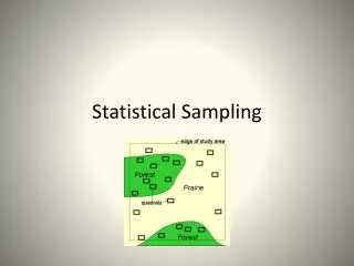
Statistical Sampling. Sampling. Simple Random Sampling. Every possible combination of sample units has an equal and independent chance of being selected. However…. Systemic Sampling. Beware coincidental bias of sample interval and natural area. Ridges River bends Etc.

Statistical Sampling
E N D
Presentation Transcript
Simple Random Sampling • Every possible combination of sample units has an equal and independent chance of being selected. • However…
Systemic Sampling • Beware coincidental bias of sample interval and natural area. • Ridges • River bends • Etc.
Stratified Random Sampling • The point is to reduce variability within strata. • Example: if you were measuring average estrogen levels in humans, you would stratify male versus female. • Can you think of some forest examples?
Sampling In Excel =AVERAGE(A1:An) mean of the squared deviations Square root of variance
Standard Deviation Use Excel function =STDEV(A1:An) or =STDEV.S(A1:An)
Exercise in Random Sampling • Student heights equals population • Calculate population mean, etc. • Take a systemic 20% sample compare estimates of population. • Take a 50% sample (systemic or random) and compare results. • Calculate mean, variance, SD and CV of both population and samples.
Variability The differences between individuals or units in a population
Standard Error of the mean • Equals the standard deviation of all possible sample means around the true population mean.
Finite Population Correction Factor The finite population correction factor serves to reduce the standard error when relatively large samples are drawn from finite populations
Confidence Interval • specify the precision of the sample mean in relation to the population mean.
Effect of Standard Deviation The red distribution has a mean of 40 and a standard deviation of 5; the blue distribution has a mean of 60 and a standard deviation of 10. For the red distribution, 68% of the distribution is between 45 and 55; for the blue distribution, 68% is between 40 and 60.
Sampling Error Rather than work with absolute confidence limits, convert them to a percent of the sample mean which is called sampling error. The notation in the handbook is an upper case E. Take the confidence interval quantity and scale it to the sample mean by dividing by the sample mean. Express this value as a percent by multiplying by 100. By expressing the confidence interval as a percentage, the mean can be plus or minus the percentage derived. For example, at 95% confidence, an estimate of the mean has a confidence interval of 46.4 plus or minus 2.6. When expressed as a sampling error percent, the mean is plus or minus 5.6% which says the true population mean falls within 95% percent of the estimate.
Determining Sample Size For a 95% confidence level, the t value approaches 2 as the sample size gets large, so a t value of 2 is commonly used when estimating sample size. The CV is the relative variability in the population being sampled. Use the population CV if known or use an estimate if it is not known. The E represents the desired sampling error, for example, 10%
Effect of CV Change As the coefficient of variation increases, so does the required sample size.
Using CV for Comparison Because CVs have no associated unit of measure, they can be useful in comparing sampling methods to determine which is most efficient. So which method of sampling would require fewer samples?
Sampling Intensity Revisited The USFS Way
Sample Selection – from Precruise data Determine the sampling error for the sale as a whole. (set to 10%) Subdivide (or stratify) the sale population into sampling components as needed to reduce the variability within the sampling strata. Calculate the coefficient of variation (CV) by stratum and a weighted CV over all strata. (this will be covered more later in the statistics lectures) Calculate number of plots for the sale as a whole and then distribute by stratum.
Number of Plots Value of t is assumed to be 2 Error is set at 10%
Distribute Plots by Stratum For each stratum, the calculation would look like this: n1 = (17.6 * 185) / 67.9 = 48 plots n2 = (7.7 * 185) / 67.9 = 21 plots n3 = (7.2 * 185) / 67.9 = 20 plots n4 = (35.4 * 185) / 67.9 = 96 plots Which totals to the 185 plots for the sale.
Tree Expansion Factor 1 divided by the fixed plot size times the number of plots
Sample Error – Step 2 36.2% is a bit larger than the level we set to begin with (10%) – Implications?