Acceptance Sampling and Statistical Process Control
Acceptance Sampling and Statistical Process Control. Probability Review. Permutations (order matters) Number of permutations of n objects taken x at a time. Probability Review. Permutations (cont.) Example: Number of permutations of 3 letters (A, B, C) taken 2 at a time

Acceptance Sampling and Statistical Process Control
E N D
Presentation Transcript
Probability Review Permutations (order matters) • Number of permutations of n objects taken x at a time
Probability Review Permutations (cont.) • Example: Number of permutations of 3 letters (A, B, C) taken 2 at a time (A,B,C) AB, BA, AC, CA, BC, CB
Probability Review Combinations (order does not matter) • Number of combinations of n objects taken x at a time
Probability Review(cont.) Combinations • Example: Number of combinations of 3 letters (A, B, C) taken 2 at a time (A, B, C) = AB, AC, BC
Probability Review Binomial Distribution • Sum of a series of independent, identically distributed Bernoulli random variables • Probability of x defectives in n items • p = probability of “success” (usually determined from long-term process average) • 1-p = probability of “failure”
Probability Review Binomial Distribution (cont.) • Example: What is the probability of 2 defectives in 4 items if p = 0.20?
Probability Review Binomial Distribution Exercises
Probability Review Hypergeometric Distribution • Random sample of size n selected from N items, where D of the N items are defective • Probability of finding r defectives in a sample of size n from a lot of size N
Probability Review Hypergeometric Distribution (cont.) • Example: What is the probability of finding 0 defects in 10 items taken from a lot of size 100 containing 4 defects?
Probability Review Hypergeometric Distribution Exercises
Probability Review • Binomial Approximation of Hypergeometric • Use when n/N 0.10 • P ~ D/N • Example: What is the probability of finding 0 defects in 10 items selected from a lot of size 100 containing 40 defects? • We got 0.652 from the straight hypergeometric.
Probability Review • Poisson Distribution (to approximate Binomial) • Use when n20 and p0.05 • =np (average number of defects) • Example: What is the probability of finding 2 defects in 4 items if p = 0.20? • We got 0.1536 with the straight Binomial.
Acceptance Sampling • Definition: process of accepting or rejecting a lot by inspecting a sample selected according to a predetermined sampling plan • Notation: N = batch size n = sample size c = acceptance number p = proportion defective (known or long-term average) Pa = probability that a batch will be accepted
and Risks • Type I Error: rejecting an acceptable lot (a.k.a. producer’s risk) P(Type I Error) = • Type II Error: accepting an unacceptable lot (a.k.a. consumer’s risk) P(Type II Error) =
Operating Characteristic (OC) Curves • OC Curves characterize acceptance sampling plans. • OC Curves are complete plotting of Pa for a lot at all possible values of p.
OC Curves • Steepness of OC curves indicates the power of the acceptance sampling plans to distinguish “good” lots from “bad” lots. Power = 1-P(accepting lot | p) = P(rejecting lot | p) • For large values of p (i.e., large number of defects), we want the Power to be large (i.e., close to 1).
OC Curves • Type A OC Curve • Uses known value for p (i.e., lot composition is known) • Can use hypergeometric distribution • Type B OC Curve • Uses process average for p • Can use binomial distribution
Acceptance Sampling Plans • Considerations: • -risk • -risk • Acceptable Quality Level (AQL) • Lot Tolerance Percent Defective (LTPD)
Acceptance Sampling Plans Acceptable Quality Level (AQL) • Maximum percent defective that is acceptable = P(rejecting lot | p = AQL) • Corresponds to higher Pa (left-hand side of OC Curve) Lot Tolerance Percent Defective (LTPD) • Worst quality that is acceptable (accepted with low probability) = P(accepting lot | p = LTPD) • Corresponds to lower Pa (right-hand side of OC Curve)
Acceptance Sampling Plans • Single Sampling • Take a single sample from the lot for inspection • Quality of sampled work determines lot decision • Double Sampling • One small sample from the lot for inspection • If quality of first sample is acceptable, that sample determines lot decision • If quality of first sample is unacceptable or not clear, select a second small sample to make lot decision
Acceptance Sampling Plans Single-Sampling vs. Double-Sampling Plans • Either plan can satisfy AQL and LTPD requirements • Double sampling often results in smaller total sample sizes • Double sampling can increase cost if second sample is required often • Psychological advantage to double sampling (second chance)
Inspection • Inspection involves verifying the quality of a work unit. • Most inspection includes rectification of errors found. • Rectification: • 100% of defective work units are repaired or replaced • Rejected lots are 100% verified and rectified • Verifiers should have higher level of understanding to establish confidence in the inspection/rectification process.
Average Outgoing Quality Average Outgoing Quality (AOQ) = proportion defective after inspection and rectification • AOQ curve relates outgoing quality to incoming quality • Average Outgoing Quality Level (AOQL) = point where outgoing quality is worst • Maximum AOQ over all possible values of p
Average Outgoing Quality Level (Table 1 provides values of y for c = 0,1,2,…,40) For small sampling fractions,
Average Outgoing Quality Level Determining sample size for desired outgoing quality (AOQL): • Given desired AOQL • Given desired acceptable number of defects, c • Given y-value from Table 1 for desired c
Average Outgoing Quality Level Determining AOQL for known sample size and desired acceptable number of rejects, c: • Given sample size, n • Given desired c-value • Given y-value from Table 1 for desired c-value • Adjust c-value and n to manipulate the AOQL
Additional Acceptance Sampling Terminology Average Sample Number (ASN) • Average number of sample units inspected to reach lot decision • In single-sampling plan: ASN = n • In double-sampling plan: n1 ASN n1 + n2
Additional Acceptance Sampling Terminology • Average Total Inspection (ATI): • Average number of units inspected per lot • In single-sampling plan: n ATI N • ATI = n + (1-Pa)(N-n) • Better incoming quality less inspection
Additional Acceptance Sampling Terminology • Average Fraction Inspected (AFI): • Average fraction of units inspected per lot • AFI = ATI/N • In single-sampling plan: n/N AFI 1
Acceptance Sampling Acceptance Sampling Plan Exercise
Other Sampling Plans • Continuous Sampling • Not possible to use lots/batches • Level of inspection depends on perceived quality level • Continuous Sampling Plan 1 (CSP1) • Start at 100% inspection • After i consecutive non-defectives, go to sample inspection • Go back to 100% inspection when a defective is found
Other Sampling Plans • Chain Sampling • Like standard sampling plans with c=0 • However, allow 1 defect in a lot if previous i lots were defective-free • Useful for small lots where c=0 is required • Skip-Lot Sampling • Lot-based continuous sampling • Lots inspected 100% until i lots are defective-free, then go to sample inspection of lots
Acceptance Sampling Trade-Off Sampling Fraction vs. Acceptance Criteria • Assuming a set quality level (AOQL), we can make choices regarding inspection rates and acceptance criteria • To decrease inspection rate, we must tighten acceptance criteria • To allow more defects, we must increase sample size
Acceptance Sampling Trade-Off • Example: Desired AOQL = 5%, Batch Size 1-800 items • 25% inspection accept if 6 or fewer defects in a sample of size 60 • 10% inspection accept if 5 or fewer defects in a sample of size 60 • See Tables 1 and 2
Creating Work Units • Homogeneity • Alike items within a batch • Helps to keep samples representative • Batch Size • Rule-of-thumb: ½ to 1 day of work • Very small batch frequent QC, more paperwork • Very large batch delayed feedback, higher rework risk
Sample Selection Important for sample selection to be completely random • Random Number Table • Number batch items 1 through N • Select random point in random number table • Use next n numbers in the table as the batch items to select
Sample Selection Systematic Sampling • Select a random start between 1 and 10 • Select every xth item until n items are selected
U.S. Census Bureau Applications Address Canvassing • Three random starts within listing pages • One random start provides start for check of total listings • Two random starts provide start for check of added housing units and deleted housing units • No errors allowed • QA form example from upcoming 2004 Census Test
U.S. Census Bureau Applications Review of Map Improvement Files • Select map “features” for QC review • Acceptance Sampling plan • Global AQL requirement • Sample size dependent on “batch” size • Acceptance number dependent on sample size • Uses stratified sampling
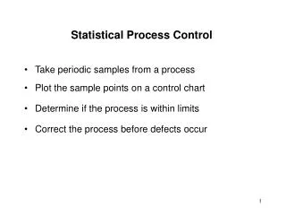
Process Control • Allows us to plan quality into our processes • Spend fewer resources on inspection and rework • Observe processes, collect samples, measure quality, determine if the process produces acceptable results
Process Control Stresses prevention over inspection • Traditional approach to QC: • Most resources spent on inspection and rework • Process Control approach to QC: • Most resources spent on prevention with relatively little spent on inspection and rework • Lower overall cost
Sources of Variation Random Sources • Cause of variation is common or unassignable • Process is still “in control” • Difficult or impossible to eliminate • Requires modification to the process itself
Sources of Variation Non-Random Sources • Cause of variation is special and assignable • Could be difficult to eliminate • Causes process to be “out of control” • Can address the specific cause of the variation
Sources of Variation Diagnosing non-random variation • “2-out-of-3” – if two out of three consecutive points are out of control • “4-out-of-5” – if four out of five consecutive points are out of control • “7 successive” – if seven consecutive points are on one side of the process average
Control Charts • Graphical device for assessing statistical control • Plots data from a process in time order • Three reference lines: • Upper Limit • Center Line (CL) • Lower Limit
Control Charts • CL represents the process average • Upper and lower limits represent the region the process moves in under random variation
Control Charts Control chart limits can be Control Limits or Specification Limits • Control Limits: based on quality capability of the process • Control limits traditionally set at 3 standard deviations away from the CL • Specification Limits: based on quality goal
Control Charts • Example: Chemical process with assumed concentration of 3%, desired concentration 3.2% and 2.8% • Specification Limits: LSL = 2.8, USL = 3.2 • Control Limits: LCL = 2.5, UCL = 3.5 (based on true capability of process)