Acceptance Sampling
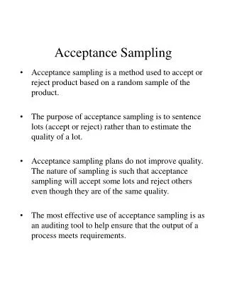
Acceptance Sampling. Acceptance sampling is a method used to accept or reject product based on a random sample of the product. The purpose of acceptance sampling is to sentence lots (accept or reject) rather than to estimate the quality of a lot.

Acceptance Sampling
E N D
Presentation Transcript
Acceptance Sampling • Acceptance sampling is a method used to accept or reject product based on a random sample of the product. • The purpose of acceptance sampling is to sentence lots (accept or reject) rather than to estimate the quality of a lot. • Acceptance sampling plans do not improve quality. The nature of sampling is such that acceptance sampling will accept some lots and reject others even though they are of the same quality. • The most effective use of acceptance sampling is as an auditing tool to help ensure that the output of a process meets requirements.
As mentioned acceptance sampling can reject “good” lots and accept “bad” lots. More formally: Producers risk refers to the probability of rejecting a good lot. In order to calculate this probability there must be a numerical definition as to what constitutes “good” • AQL (Acceptable Quality Level) - the numerical definition of a good lot. The ANSI/ASQC standard describes AQL as “the maximum percentage or proportion of nonconforming items or number of nonconformities in a batch that can be considered satisfactory as a process average” • Consumers Risk refers to the probability of accepting a bad lot where: • LTPD (Lot Tolerance Percent Defective) - the numerical definition of a bad lot described by the ANSI/ASQC standard as “the percentage or proportion of nonconforming items or noncomformities in a batch for which the customer wishes the probability of acceptance to be a specified low value.
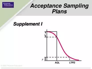
The Operating Characteristic Curve is typically used to represent the four parameters (Producers Risk, Consumers Risk, AQL and LTPD) of the sampling plan as shown below where the P on the x axis represents the percent defective in the lot: • Note: if the sample is less than 20 units the binomial distribution is used to build the OC Curve otherwise the Poisson distribution is used.
Designing Sampling Plans • Operationally, three values need to be determined before a sampling plan can be implemented (for single sampling plans): • N = the number of units in the lot • n = the number of units in the sample • c = the maximum number of nonconforming units in the sample for which the lot will be accepted. • While there is not a straightforward way of determining these values directly given desired values of the parameters, tables have been developed. Below is an excerpt of one of these tables.
Three alternatives for specifying sampling plans • Producers Risk and AQL specified • Consumers Risk and LTPD specified • All four parameters specified • For the first two cases we simply choose the acceptance number and divide the appropriate column by the associated parameter to get the sample size. • Example 1: Given a producers risk of .05 and an AQL of .015 determine a sampling plan • c = 1: n = .355/.015 ~ 24 • c = 4: n = 1.97/.015 ~ 131 • Example 2: Given a consumers risk of .1 and a LTPD of .08 determine a sampling plan • c = 0: n = 2.334/.08 ~ 29 • c = 5: n = 9.274/.08 ~ 116 • Note: you can check these with the OC curve posted on my web site
All four parameters specified • When all four parameters are specified we must first find a value close to the ratio LTPD/AQL in the table. Then values of n and c are found. • Example: Given producers risk of .05, consumers risk of .1, LTPD 4.5%, and AQL of 1% find a sampling plan. • Since 4.5/1 = 4.5 is between c= 3 and c = 4. Using the n(AQL) column the sample sizes suggested are 137 and 197 respectively. Note using this column will ensure a producers risk of .05. Using the n(LTPD) column will ensure a consumers risk of .1
Double Sampling • In an effort to reduce the amount of inspection double (or multiple) sampling is used. Whether or not the sampling effort will be reduced depends on the defective proportions of incoming lots. Typically, four parameters are specified: n1 = number of units in the first sample c1 = acceptance number for the first sample n2 = number of units in the second sample c2 = acceptance number for both samples
Procedure • A double sampling plan proceeds as follows: A random sample of size n1 is drawn from the lot. If the number of defective units (say d1 ) c1 the lot is accepted. If d1 c2 the lot is rejected. If neither of these conditions are satisfied a second sample of size n2 is drawn from the lot. If the number of defectives in the combined samples (d1 + d2) > c2 the lot is rejected. If not the lot is accepted.
Example • Consider a double sampling plan with n1 = 50; c1 = 1; n2 = 100; c2 = 3. What is the probability of accepting a lot with 5% defective? • The probability of accepting the lot, say Pa, is the sum of the probabilities of accepting the lot after the first and second samples (say P1 and P2) • To calculate P1 we first must determine the expected number defective in the sample (50*.05) we can then use the Poisson function to determine the probability of finding 1 or fewer defects in the sample, e.g., Poisson(1,2.5,true) = .287 • To calculate P2 we need to determine first the scenarios that would lead to requiring a second sample. Then for each scenario we must determine the probability of acceptance. P2 will then be the some of the probability of acceptance for each scenario.
Example continued • For this example, there are only two possible scenarios that would lead to requiring a second sample: • Scenario 1: 2 nonconforming items in the first sample • Scenario2: 3 nonconforming items in the first sample. • The probability associated with these two scenarios is found as follows: • P(scenario 1) = Poisson(2,2.5,false) = .257 • P(scenario 2) = Poisson(3,2.5,false) = .214 • Under scenario 1 the lot will be accepted if there are either 1 or 0 nonconforming items in the second sample. The expected number of nonconforming items in the second sample .05(100) = 5 • the probability is then: Poisson(1,5,true) = .04 • therefore the probability of acceptance under scenario 1 is (.257)*(.04) = .01 • Under scenario 2 we will accept the lot only if there are 0 nonconforming items in the second sample, i.e., Poisson(0,5,false) = .007 • therefore the probability of acceptance under scenario 2 is (.214)*(.007) = .0015 • so the probability of acceptance on the second sample is .01 + .0015 = .0115 • So the overall probability of acceptance is (probability of acceptance on first sample + probability of accepting after 2 samples) = .287 + .0115 = .299
Average Sample Number • Since the goal of double sampling is to reduce the inspection effort, the average number of units inspected is of interest. This is easily calculated as follows • Let PI = the probability that a lot disposition decision is made on the first sample, i.e., (probability that the lot is rejected on the first sample + probability that the lot is accepted on the first sample) • Then the average number of items is: n1(PI) +(n1 + n2)(1 - PI) = n1 + n2(1 - PI)
The average sample number curve can be derived from the data on the OC chart