Understanding Attribute Acceptance Sampling
Understanding Attribute Acceptance Sampling. Dan O’Leary CBA, CQA, CQE, CRE, SSBB, CIRM President Ombu Enterprises, LLC Dan@OmbuEnterprises.com www.OmbuEnterprises.com 603-358-3082. OMBU ENTERPRISES, LLC. © 2009, 2010 Ombu Enterprises, LLC. Outline. Sampling Plan Concepts ANSI/ASQ Z1.4

Understanding Attribute Acceptance Sampling
E N D
Presentation Transcript
Understanding Attribute Acceptance Sampling Dan O’Leary CBA, CQA, CQE, CRE, SSBB, CIRM President Ombu Enterprises, LLC Dan@OmbuEnterprises.com www.OmbuEnterprises.com 603-358-3082 OMBU ENTERPRISES, LLC © 2009, 2010 Ombu Enterprises, LLC Attribute Sampling
Outline • Sampling Plan Concepts • ANSI/ASQ Z1.4 • Single Sampling Plans • Double and Multiple Sampling Plans • c=0 Sampling Plans • Summary and Conclusions • Questions Attribute Sampling
Sampling Plans Some Initial Concepts Attribute Sampling
A Typical Application • You receive a shipment of 5,000 widgets from a new supplier. • Is the shipment good enough to put into your inventory? How will you decide? Attribute Sampling
You Have a Few Approaches • Consider three potential solutions • Look at all 5,000 widgets (100% inspection) • Don’t look at any, put the whole shipment into stock (0% inspection) • Look at some of them, and if enough of those are good, keep the lot (Acceptance sampling) • In a sampling plan, we need to know: • How many to inspect or test? • How to distinguish “good” from “bad”? • How many “good” ones are enough? Attribute Sampling
Attributes We classify things using attributes A stop light can be one of three colors: red, yellow, or green The weather can be sunny, cloudy, raining, or snowing A part can be conforming or nonconforming Variables We measure things using variables The temperature of the oven is 350° F The tire pressure is 37 pounds per square inch (psi). The critical dimension for this part number is 3.47 inches. Two Kinds of Information Attribute Sampling
Convert Variables To Attributes • Consider an important dimension with a specification of 3.5±0.1 inches. • Piece A, at 3.56 inches is conforming. • Piece B, at 3.39 inches is nonconforming. LSL Target USL B A 3.4” 3.5” 3.6” Specification is 3.5±0.1 Attribute Sampling
A Note About Language • Avoid “defect” or “defective” • They are technical terms in the quality profession, with specific meaning • They are also technical terms in product liability, with a different meaning • They have colloquial meaning in ordinary language • I encourage the use of “nonconformances” or “nonconforming” Attribute Sampling
Two Attribute Sampling Plans • ANSI/ASQ Z1.4 Sampling Procedures and Tables for Inspection By Attributes • ISO 2859-1 Sampling procedures for inspection by attributes – Part 1: Sampling schemes indexed by acceptance quality limit (AQL) for lot-by-lot inspection • ANSI/ASQ Z1.4 and ISO 2859-1 are the classical methods evolved from MIL-STD-105 • The c=0 plans are described in Zero Acceptance Number Sampling Plans by Squeglia Attribute Sampling
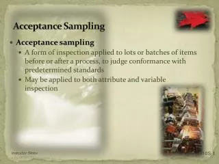
Acceptance Sampling is Common . . . • The most common place for acceptance sampling is incoming material • A supplier provides a shipment, and we judge its quality level before we put it into stock. • Acceptance sampling (with rectifying inspection) can help protect from processes that are not capable • Destructive testing is also a common application of sampling Attribute Sampling
. . . Acceptance sampling isn’t always appropriate • Acceptance sampling is not process control • Statistical process control (SPC) is the preferred method to prevent nonconformances. • Think of SPC as the control method, and acceptance sampling as insurance • You practice good driving techniques, but you don’t cancel your insurance policy Attribute Sampling
Attribute Sampling Plans Single Sample Example Attribute Sampling
We start with an exercise, and then explain how it works • Your supplier submits a lot of 150 widgets and you subject it to acceptance sampling by attributes. • The inspection plan is to select 20 widgets at random. • If 2 or fewer are nonconforming, then accept the shipment. • If 3 or more are nonconforming, then reject the shipment. In symbols: N =150 n = 20 c = 2, r = 3 This is a Z1.4 plan that we will examine. Attribute Sampling
Here is the basic approach • Select a singlesimplerandomsample of n = 20 widgets. • Classify each widget in the sample as conforming or nonconforming (attribute) • Count the number of nonconforming widgets • Make a decision (accept or reject) on the shipment • Record the result (quality record) Attribute Sampling
Attribute Sampling Plans ANSI/ASQ Z1.4 Attribute Sampling
Current status of the standards • MIL-STD-105 • The most recently published version is MIL-STD-105E • Notice 1 cancelled the standard and refers DoD users to ANSI/ASQC Z1.4-1993 • ANSI/ASQ Z1.4 • Current version is ANSI/ASQ Z1.4: 2008 • FDA Recognition • The FDA recognizes ANSI/ASQ Z1.4-2008 as a General consensus standard • Extent of Recognition: Use of all Single, Double and Multiple sampling plans according to the standard's switching rules to make acceptance/rejection decisions on a continuous stream of lots for a specified Acceptance Quality Limit (AQL). Attribute Sampling
Getting started with Z1.4 • To correctly use Z1.4, you need to know 5 things • Lot Size • Inspection Level • Single, Double, or Multiple Sampling • Lot acceptance history • AQL Attribute Sampling
The Flow of Information We develop our example in these boxes, by showing the choice we make. Lot Size Code Letter (Tbl. I) Inspection Level Table II, III, or IV S/D/M Sub-table A, B, or C N/R/T Sampling Plan ni, ci, & ri Traditional Information Sources Purchasing – Lot Size Quality Engineer – Inspection Level, S/D/M, AQL Lot History – N/R/T AQL Attribute Sampling
Lot Size • The lot size is the number of items received at one time from the supplier. • For incoming inspection, think of it as the quantity on the pack slip. • The Purchase Order (or contract) typically sets the lot size. Received 150 pieces N = 150 Attribute Sampling
Inspection Level • The inspection level determines how the lot size and the sample size are related • Z1.4 provides seven different levels: S1, S2, S3, S4, I, II, and III. • Use Inspection Level II unless you have a compelling reason to do something else. • The Quality Engineer sets the Inspection Level. Use Level II Attribute Sampling
Code Letter • The Inspection Level and Lot Size combine to determine the code letter. • Use Table I to determine the code letter. Lot Size Level II Lot Size = 150 Code Letter = F Code Letter (Tbl. I) Inspection Level Attribute Sampling
Single, Double, or Multiple Sampling (S/D/M) • Decide the type of sampling plan (Single, Double, or Multiple) • This is a balance between average sample number (ASN) and administrative difficulty. • Generally, moving from single to double to multiple • The ASN goes down • The administrative difficulty goes up Use Single Sampling Table II Code Letter (Tbl. I) Table II, III, or IV S/D/M Attribute Sampling
Lot acceptance history • Z1.4 uses a system of switching rules • Based on the lot history, we inspect the same (normal), less (reduced), or more (tightened). Table II, III, or IV Sub-table A, B, or C N/R/T Attribute Sampling
Inspection States • The system can be in one of four states: • Normal • Reduced • Tightened or • Discontinue Use Normal Attribute Sampling
AQL • We will discuss AQL shortly • Z1.4 uses the AQL to index the sampling plans. • The supplier’s process average should be as low as possible, but certainly less than the Z1.4 AQL. • The Quality Engineer sets the AQL. Use AQL of 4.0 Attribute Sampling
Sampling Plan • The type and history get us to the right table. • The Code Letter and AQL get us to the sampling plan. • Note, however, that you may have to use the “sliders” to get the sampling plan. Sample Size = 20 Accept on 2 Reject on 3 Sub-table A, B, or C Sampling Plan ni, ci, & ri AQL Attribute Sampling
The Sliders • Sometimes the Code Letter, Level, and AQL don’t have a plan. • Z1.4 will send you a different plan using the “sliders” These are arrows pointing up or down. • Use the new plan (with the new code letter, sample size, accept number, and reject number). • Example: Code letter D & AQL=4.0 doesn’t have a plan • “Slide” down to N=13, Ac=1, Re = 2 Attribute Sampling
Changing the lot size • You supplier has been shipping 150 units in the lot, based on the Purchase Order, for a long time. • Your supplier calls your buyer and says, “We were near the end of a raw material run, and made 160 widgets, instead of 150. Can I ship all 160 this time?” • The buyer says, “Sure no problem. I’ll send a PO amendment.” • What is the sampling plan? • Answer: n = 32, c = 3, r = 4 The Code Letter becomes G Sample Size = 32 Accept on 3 Reject on 4 Attribute Sampling
Sampling Schemes • Z1.4 tracks the history of lot acceptance and the sampling plans as a result. • Consistently good history can reduce the sample size • Consistently poor history can shift the OC Curve • The figure is a simplified version of the switching rules Attribute Sampling
An Example of Switching Rules • Look at the handout called “Attribute Sampling Log” • This is a hypothetical example of how to keep track of the inspection history • We will follow the history to see an application of the switching rules Attribute Sampling
Sampling Some Common Concepts Attribute Sampling
Sampling With/Without Replacement • When we took the widget sample, we didn’t put them back into the lot during sampling, i.e., we didn’t replace them. • This changes the probabilities of the rest of the lot. • If the lot is large, it doesn’t make too much difference. • For small lots we need the hypergeometric distribution for the calculation. • In acceptance sampling we sample without replacement! Attribute Sampling
Simple v. Stratified Sampling • Assume the lot has N items • In a simple random sample each piece in the lot has equal probability of being in the sample. • In a stratified sample, the lot is divided into H groups, called strata. Each item in the lot is in one and only one stratum. • You receive a shipment of 5,000 AAA batteries in 50 boxes of 100 each. • First you take a sample of the boxes, then you take a sample of the batteries in the sampled boxes • This is a stratified sample: N=5,000 & H=50. Attribute Sampling
Our Conventions • Unless we say otherwise we make the following conventions • Sampling is performed without replacement • Sampling is a simple random sample Attribute Sampling
The Binomial Distribution Attribute Sampling
Bernoulli Trial • Bernoulli trials are a sequence of nindependent trials, where each trial has only two possible outcomes. • Example – Flip a coin fifty times • This is a sequence of trials • n = 50 • The trials are independent, because the coin doesn't “remember” the previous trial • The only outcome of each trial is a head or a tail Attribute Sampling
The Binomial Distribution • The Bernoulli trial has two possible outcomes. • One outcome is “success” with probability p. • The other “failure” with probability q = 1 – p. • The binomial distribution is the probability of x successes in n trials Attribute Sampling
Excel Example n = 20, p = 0.1 What is the probability of exactly 0 successes, 1 success, etc. BINOMDIST(number_s,trials,probability_s,cumulative) Attribute Sampling
Attribute Sampling Plans Single Sample Plans Attribute Sampling
Attribute Sampling Plans • Single sample plans – Take one sample selected at random and make an accept/reject decision based on the sample • Double sample plans – Take one sample and make a decision to accept, reject, or take a second sample. If there is second sample, use both to make an accept/reject decision. • Multiple sample plans – Similar to double sampling, but more than two samples are involved. Attribute Sampling
The AQL concept • The AQL is the poorest level of quality (percent nonconforming) that the process can tolerate. • The input to this process (where I inspect) is defined as: • The supplier produces product in lots • The supplier uses essentially the same production process for each lot • The supplier’s production process should run as well as possible, i.e., the process average nonconforming should be as low as possible • This “poorest level” is the acceptable quality level or AQL. Attribute Sampling
The intentions of the AQL • The AQL provides a criterion against which to judge lots. • It does not . . . • Provide a process or product specification • Allow the supplier to knowingly submit nonconforming product • Provide a license to stop continuous improvement activities Attribute Sampling
The relationship between process control and acceptance sampling Producer Consumer Production Process Acceptance Process Control Method Attribute Sampling AQL = 4.0% Use Z1.4 Single Sample Level II Control Method SPC: p-chart Standard given: p0 = 0.02 Central Line: p0 = 0.02 Control Limits: Attribute Sampling
What Does AQL Mean? • If the supplier’s process average nonconforming is below the AQL, the consumer will accept all the shipped lots. • If the supplier’s process average nonconforming is above the AQL, the consumer will reject all the shipped lots. Illustrates an AQL of 4.0% Ideal OC curve Attribute Sampling
Sampling Doesn’t Realize The Ideal OC Curve Increasing n (with c proportional) approaches the ideal OC curve. Increasing c (with n constant) approaches the ideal OC curve. Attribute Sampling
Consider Four Possible Outcomes Producer’s Risk – The probability of rejecting a “good” lot. Consumer’s Risk – The probability of accepting a “bad” lot. Attribute Sampling
Specific Points on the OC Curve The Producer’s Risk has a value of α. The point (p1, 1-α) shows the probability of accepting a lot with quality p1. The OC curve for N = 150, n = 20, c = 2 The Consumer’s Risk has a value of β. The point (p2, β) shows the probability of accepting a lot with quality p2. The point (p3, 0.5) shows the probability of acceptance is 0.5. Attribute Sampling
Some Conventions • Some conventions for these points include: • α = 5% and β = 5% • The point (p1, 1-α) = (AQL, 95%) • The point (p2, β) = (RQL, 5%) • We also see α = 5% and β = 10% • The point (p1, 1-α) = (AQL, 95%) • The point (p2, β) = (RQL, 10%) • Z1.4 doesn’t adopt these conventions Attribute Sampling
The Previous OC Curve With The Points Named Attribute Sampling
Characterizing Attribute Sampling Plans • We typically use four graphs to tell us about a sampling plan. • The Operating Characteristic (OC) curve • The probability of acceptance for a given quality level. • The Average Sample Number (ASN) curve • The expected number of items we will sample (most applicable to double, multiple, and sequential samples) • The Average Outgoing Quality (AOQ) curve • The expected fraction nonconforming after rectifying inspection for a given quality level. • The Average Total Inspected (ATI) curve • The expected number of units inspected after rectifying inspection for a given quality level. Attribute Sampling