Acceptance Sampling Plans by Variables
Acceptance Sampling Plans by Variables. CH 16. Contents. Advantages and Disadvantages of Acceptance Sampling by Variables. Types of Acceptance Sampling by Variables. Chain Sampling. Continuous Sampling. Advantages of Variables Sampling.

Acceptance Sampling Plans by Variables
E N D
Presentation Transcript
Contents • Advantages and Disadvantages of Acceptance Sampling by Variables. • Types of Acceptance Sampling by Variables. • Chain Sampling. • Continuous Sampling.
Advantages of Variables Sampling • The same OC curve can be obtained with a smaller sample size than would be required by an attributes sampling plan. • Measurement data provide more information about the manufacturing process. • When AQLs are very small, the sample sizes required by attributes sampling plans are very large.
Disadvantages of Variables Sampling • The distribution of the quality characteristic must be known. • A separate sampling plan must be employed for each quality characteristic that is being inspected.
Types of Variables Sampling Plans • Plans that control the lot or process fraction defective. • Plans that control a lot or process mean.
Plans to Control Process Fraction Defective • Since the quality characteristic is a variable, there will exist either LSL, USL, or both, that define the acceptable values of this parameter. • Fig. 1 illustrates the situation in which the quality characteristic x is normally distributed and there is LSL on this parameter. Fig. (1)
Plans to Control Process Fraction Defective • Procedure 1 (k-Method) • Take a random sample of n items from the lot and compute • If there is a critical value of p of interest that should not be exceeded with stated probability, we can translate this value of p into critical distance k. • If ZLSL≥ k, we would accept the lot because the sample data imply that the lot mean is sufficiently far above LSL to insure that p is satisfactory.
Plans to Control Process Fraction Defective • Procedure 2 (M-Method) • Compute ZLSL . • Use ZLSL to estimate the fraction defective of the lot or process . • Determine the max. allowable fraction defective M (using specific values of n, k). • If exceeds M, reject the lot; otherwise, accept it.
Plans to Control Process Fraction Defective • Notes • In the case of an USL, we compute • If is unknown, it is estimated by s. • When there is only a single specification limit (LSL or USL), either procedure may be used. • When there are both LSL and USL, M-method should be used by computing ZLSL and ZUSL, finding the correspondingfraction defective estimates and Then, if + ≤ M, the lot will be accepted. ^ ^ pLSL pUSL ^ ^ pLSL pUSL
Designing a variables sampling plan with a specified OC curve • Let be the two points on the OC curve of interest. • are the levels of lot or process fraction nonconforming that correspond to acceptable and rejectable levels of quality, respectively. p1and p2
Designing a variables sampling plan with a specified OC curve • Example 1
Designing a variables sampling plan with a specified OC curve
Designing a variables sampling plan with a specified OC curve • Example 2 :Design a sampling plan using M-method
Designing a variables sampling plan with a specified OC curve
MIL STD 414 • There are five general levels of inspection, and level IV is designated as “normal”.
MIL STD 414 • As MIL STD 105E, sample size code letters are used, but the same code letter does not imply the same sample size in both standards. • Sample sizes are a function of the lot size and the inspection level. • All the sampling plans in the standards assume that the quality characteristic is normally distributed.
MIL STD 414 • Organization of MIL STD 414
MIL STD 414 • Example 3: Using MIL STD 414 Solution From table, if we use IV level, the sample size code letter is O. From a second table, we find n=100. For AQL of 1%, on normal inspection, k=2. For AQL of 1%, on tightened inspection, k=2.14
Plans to Control A Process Mean • Example 4 Solution Let XA be the value of the sample average below witch the lot will be accepted. If lots have 0.95 probability of acceptance, then P (X ≤ XA ) = 0.95 - -
Plans to Control A Process Mean P (Z≤ ) =0.95 =1.64 If lots have 0.1 probability of acceptance, then P (X ≤ XA ) = 0.1 p (Z ≤ ) = 0.1 = -1.28 These two equations can be solved for n and XA , giving n=9 and XA=0.356 - - -
Chain Sampling Plan • It is used for small sample size plans that have acceptance number of zero. • Lots should be produced under the same conditions, and be expected to be of the same quality. • There should be a good record of quality performance on the part of supplier. • The general procedure for ChSP-1: • For each lot, select the sample of size n and observe the defectives. • If sample has zero defectives, accept the lot . • If sample has two or more defectives, reject the lot. • If sample has 1 defective, accept the lot provided that there have been no defectives in the previous i lots.
Chain Sampling Plan • The effect of chain sampling on OC curve: • It is more difficult to reject lots with very small p with ChSp-1 Plan than it is with ordinary single Plan. • In practice, values of i vary between 3 and 5, since OC curves of such plans approximate OC curve for S-S plan. • The points on the OC curve of a ChSP-1 plan are given by:
Continuous Sampling Plan • Used when production is continuous. That is, the manufacturing operation do not result in the natural formation of lots. • It consists of altering sequences of sampling inspection and screening (100% inspection).
Continuous Sampling Plan • Procedure for CSP-1 plans
Continuous Sampling Plan • The average number of units inspected in a 100% screening is equal to , where q=1-p • The average number of units passed under the sampling inspection is • The average fraction of total manufactured units inspected in the long run is • The average fraction of manufactured units passed under the sampling procedure is
Continuous Sampling Plan • OC curves for various continuous sampling plans, CSP-1.