Acceptance Sampling Plans
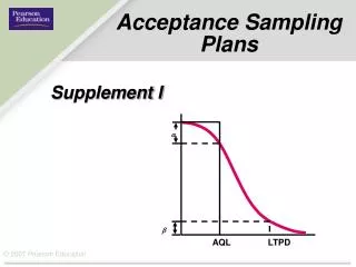
a. . AQL LTPD. Acceptance Sampling Plans. Supplement I. Acceptance Sampling. Acceptance sampling is a statistical process for determining whether to accept or reject a lot of products by testing a random sample of parts taken from the lot.

Acceptance Sampling Plans
E N D
Presentation Transcript
a AQL LTPD Acceptance Sampling Plans Supplement I
Acceptance Sampling • Acceptance sampling is a statistical process for determining whether to accept or reject a lot of products by testing a random sample of parts taken from the lot. • An acceptance sampling plan is specified by n and c, where, • n = the sample size, and • c = the critical number of defectives in the sample up to which the lot will be accepted.
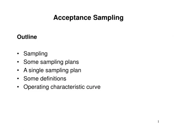
OC Curve • Let Pd = Probability of defectives in the lot • Pa = Probability of accepting the lot P(x< c), where x = number of defectives in the sample • OC Curve is a graph with values of Pd on the x-axis and the corresponding values of Pa in the y-axis.
Computing Pa for a given sampling plan and Pd value • Compute nPd • Use Poisson Probability Table and lookup the value of Pa for the value of c • Example: Given a sampling plan of n = 60 and c = 2, if Pd = 1%, nPd = 60(.01) = .6 np 0 1 2 .40 .670 .938 .992 .45 .638 .925 .989 .50 .607 .910 .986 .55 .577 .894 .982 .60 .549 .878 .977 .65 .522 .861 .972 Pa = .977
OC Curve 1.0 – 0.9 – 0.8 – 0.7 – 0.6 – 0.5 – 0.4 – 0.3 – 0.2 – 0.1 – 0.0 – Probability of acceptance | | | | | | | | | | 1 2 3 4 5 6 7 8 9 10 Proportion defective (hundredths)
Constructing OC Curve The Noise King Muffler Shop, a high-volume installer of replacement exhaust muffler systems, just received a shipment of 1,000 mufflers. The sampling plan for inspecting these mufflers calls for a sample size n=60 and an acceptance number c=1. Construct the OC curve for this sampling plan.
Probability Proportion of c or less defective defects (p) np (Pa) Comments n = 60 c = 1 Constructing an OC CurveExample I.1 1.0 – 0.9 – 0.8 – 0.7 – 0.6 – 0.5 – 0.4 – 0.3 – 0.2 – 0.1 – 0.0 – Probability of acceptance | | | | | | | | | | 1 2 3 4 5 6 7 8 9 10 Proportion defective (hundredths)
np 0 1 2 .05 .951 .999 1.000 .10 .905 .995 1.000 .15 .861 .990 .999 .20 .819 .982 .999 .25 .779 .974 .998 .30 .741 .963 .996 .35 .705 .951 .994 .40 .670 .938 .992 .45 .638 .925 .989 .50 .607 .910 .986 .55 .577 .894 .982 .60 .549 .878 .977 .65 .522 .861 .972 Probability Proportion of c or less defective defects (p) np (Pa) Comments n = 60 c = 1 Constructing an OC CurveExample I.1 1.0 – 0.9 – 0.8 – 0.7 – 0.6 – 0.5 – 0.4 – 0.3 – 0.2 – 0.1 – 0.0 – Probability of acceptance | | | | | | | | | | 1 2 3 4 5 6 7 8 9 10 Proportion defective (hundredths)
np 0 1 2 .05 .951 .999 1.000 .10 .905 .995 1.000 .15 .861 .990 .999 .20 .819 .982 .999 .25 .779 .974 .998 .30 .741 .963 .996 .35 .705 .951 .994 .40 .670 .938 .992 .45 .638 .925 .989 .50 .607 .910 .986 .55 .577 .894 .982 .60 .549 .878 .977 .65 .522 .861 .972 Probability Proportion of c or less Defective defects (p) np (Pa) Comments 0.01 0.6 Constructing an OC CurveExample I.1 n = 60 c = 1 1.0 – 0.9 – 0.8 – 0.7 – 0.6 – 0.5 – 0.4 – 0.3 – 0.2 – 0.1 – 0.0 – Probability of acceptance | | | | | | | | | | 1 2 3 4 5 6 7 8 9 10 Proportion defective (hundredths)
np 0 1 2 .05 .951 .999 1.000 .10 .905 .995 1.000 .15 .861 .990 .999 .20 .819 .982 .999 .25 .779 .974 .998 .30 .741 .963 .996 .35 .705 .951 .994 .40 .670 .938 .992 .45 .638 .925 .989 .50 .607 .910 .986 .55 .577 .894 .982 .60 .549 .878 .977 .65 .522 .861 .972 Probability Proportion of c or less defective defects (p) np (Pa) Comments n = 60 c = 1 0.01 0.6 0.878 Constructing an OC CurveExample I.1 1.0 – 0.9 – 0.8 – 0.7 – 0.6 – 0.5 – 0.4 – 0.3 – 0.2 – 0.1 – 0.0 – Probability of acceptance | | | | | | | | | | 1 2 3 4 5 6 7 8 9 10 Proportion defective (hundredths)
np 0 1 2 .05 .951 .999 1.000 .10 .905 .995 1.000 .15 .861 .990 .999 .20 .819 .982 .999 .25 .779 .974 .998 .30 .741 .963 .996 .35 .705 .951 .994 .40 .670 .938 .992 .45 .638 .925 .989 .50 .607 .910 .986 .55 .577 .894 .982 .60 .549 .878 .977 .65 .522 .861 .972 Probability Proportion of c or less defective defects (p) np (Pa) Comments n = 60 c = 1 0.01 0.6 0.878 Constructing an OC CurveExample I.1 1.0 – 0.9 – 0.8 – 0.7 – 0.6 – 0.5 – 0.4 – 0.3 – 0.2 – 0.1 – 0.0 – Probability of acceptance | | | | | | | | | | 1 2 3 4 5 6 7 8 9 10 Proportion defective (hundredths)
Probability Proportion of c or less defective defects (p) np (Pa) Comments n = 60 c = 1 0.01 0.6 0.878 Constructing an OC CurveExample I.1 1.0 – 0.9 – 0.8 – 0.7 – 0.6 – 0.5 – 0.4 – 0.3 – 0.2 – 0.1 – 0.0 – Probability of acceptance | | | | | | | | | | 1 2 3 4 5 6 7 8 9 10 Proportion defective (hundredths)
1.0 – 0.9 – 0.8 – 0.7 – 0.6 – 0.5 – 0.4 – 0.3 – 0.2 – 0.1 – 0.0 – Probability Proportion of c or less defective defects (p) np (Pa) Comments n = 60 c = 1 0.663 0.01 0.6 0.878 0.02 1.2 0.663 0.03 1.8 0.463 0.04 2.4 0.308 0.05 3.0 0.199 0.06 3.6 0.126 0.07 4.2 0.078 0.08 4.8 0.048 0.09 5.4 0.029 0.10 6.0 0.017 Probability of acceptance 0.308 0.199 0.048 | | | | | | | | | | 1 2 3 4 5 6 7 8 9 10 (AQL) (LTPD) Proportion defective (hundredths) Constructing an OC CurveExample I.1
Constructing an OC CurveExample I.1 1.0 – 0.9 – 0.8 – 0.7 – 0.6 – 0.5 – 0.4 – 0.3 – 0.2 – 0.1 – 0.0 – 0.878 0.663 Probability of acceptance 0.463 0.308 0.199 0.126 0.078 0.048 0.029 | | | | | | | | | | 1 2 3 4 5 6 7 8 9 10 0.017 Proportion defective (hundredths)
AQL and LTPD • Acceptable Quality Level (AQL) • The poorest level of quality that is acceptable to the customer. It is specified as a percentage of defectives in the lot. • Lot Tolerance Percent Defective (LTPD) • The quality level at which the lot is considered bad. It is specified as a percentage of defectives in the lot.
Risks • Producer’s risk • The probability of rejecting a good lot (i.e. Pd = AQL) based on the acceptance sampling plan. This is also known as Type I error (a). • Consumer’s risk • The probability of accepting a bad lot (i.e. Pd = LTPD) based on the acceptance sampling plan. This also known as Type II error (b).
1.0 – 0.9 – 0.8 – 0.7 – 0.6 – 0.5 – 0.4 – 0.3 – 0.2 – 0.1 – 0.0 – Probability Proportion of c or less defective defects (p) np (Pa) Comments n = 60 c = 1 0.663 0.01 (AQL) 0.6 0.878 a = 1.000 – 0.878 = 0.122 0.02 1.2 0.663 0.03 1.8 0.463 0.04 2.4 0.308 0.05 3.0 0.199 0.06 (LTPD) 3.6 0.126 b = 0.126 0.07 4.2 0.078 0.08 4.8 0.048 0.09 5.4 0.029 0.10 6.0 0.017 Probability of acceptance 0.308 0.199 0.048 | | | | | | | | | | 1 2 3 4 5 6 7 8 9 10 (AQL) (LTPD) Proportion defective (hundredths) Consumer’s and Producer’s risks - Example I.1
1.0 – 0.9 – 0.8 – 0.7 – 0.6 – 0.5 – 0.4 – 0.3 – 0.2 – 0.1 – 0.0 – a = 0.122 0.878 0.663 Probability of acceptance 0.463 0.308 0.199 0.126 0.078 0.048 0.029 b = 0.126 | | | | | | | | | | 1 2 3 4 5 6 7 8 9 10 0.017 (AQL) (LTPD) Proportion defective (hundredths) Constructing an OC CurveExample I.1
Drawing the OC CurveApplication I.1 Finding (probability of rejecting AQL quality: Cumulative Poisson Probabilities p = .03 0.965 Pa= np = 5.79 = 1 – .965 = 0.035
Drawing the OC CurveApplication I.1 Finding (probability of accepting LTPD quality: Cumulative Poisson Probabilities p = .08 0.10 Pa= np = 15.44 = Pa= 0.10
Producer’s Consumer’s Risk Risk n (p = AQL) (p = LTPD) Understanding Changes in the OC Curve (with c = 1) 1.0 – 0.9 – 0.8 – 0.7 – 0.6 – 0.5 – 0.4 – 0.3 – 0.2 – 0.1 – 0.0 – Probability of acceptance | | | | | | | | | | 1 2 3 4 5 6 7 8 9 10 (AQL) (LTPD) Proportion defective (hundredths)
Producer’s Consumer’s Risk Risk n (p = AQL) (p = LTPD) 60 0.122 0.126 Understanding Changes in the OC Curve (with c = 1) 1.0 – 0.9 – 0.8 – 0.7 – 0.6 – 0.5 – 0.4 – 0.3 – 0.2 – 0.1 – 0.0 – Probability of acceptance | | | | | | | | | | 1 2 3 4 5 6 7 8 9 10 (AQL) (LTPD) Proportion defective (hundredths)
Producer’s Consumer’s Risk Risk n (p = AQL) (p = LTPD) 60 0.122 0.126 80 0.191 0.048 Understanding Changes in the OC Curve (with c = 1) 1.0 – 0.9 – 0.8 – 0.7 – 0.6 – 0.5 – 0.4 – 0.3 – 0.2 – 0.1 – 0.0 – Probability of acceptance | | | | | | | | | | 1 2 3 4 5 6 7 8 9 10 (AQL) (LTPD) Proportion defective (hundredths)
Producer’s Consumer’s Risk Risk n (p = AQL) (p = LTPD) 60 0.122 0.126 80 0.191 0.048 100 0.264 0.017 Understanding Changes in the OC Curve (with c = 1) 1.0 – 0.9 – 0.8 – 0.7 – 0.6 – 0.5 – 0.4 – 0.3 – 0.2 – 0.1 – 0.0 – Probability of acceptance | | | | | | | | | | 1 2 3 4 5 6 7 8 9 10 (AQL) (LTPD) Proportion defective (hundredths)
Producer’s Consumer’s Risk Risk n (p = AQL) (p = LTPD) 60 0.122 0.126 80 0.191 0.048 100 0.264 0.017 120 0.332 0.006 Understanding Changes in the OC Curve (with c = 1) 1.0 – 0.9 – 0.8 – 0.7 – 0.6 – 0.5 – 0.4 – 0.3 – 0.2 – 0.1 – 0.0 – Probability of acceptance | | | | | | | | | | 1 2 3 4 5 6 7 8 9 10 (AQL) (LTPD) Proportion defective (hundredths)
Operating Characteristic Curves (with c = 1) 1.0 – 0.9 – 0.8 – 0.7 – 0.6 – 0.5 – 0.4 – 0.3 – 0.2 – 0.1 – 0.0 – n = 60, c = 1 n = 80, c = 1 n = 100, c = 1 Probability of acceptance n = 120, c = 1 | | | | | | | | | | 1 2 3 4 5 6 7 8 9 10 (AQL) (LTPD) Proportion defective (hundredths)
Producer’s Consumer’s Risk Risk c (p = AQL) (p = LTPD) Understanding Changes in the OC Curve (with n = 60) 1.0 – 0.9 – 0.8 – 0.7 – 0.6 – 0.5 – 0.4 – 0.3 – 0.2 – 0.1 – 0.0 – Probability of acceptance | | | | | | | | | | 1 2 3 4 5 6 7 8 9 10 (AQL) (LTPD) Proportion defective (hundredths)
Producer’s Consumer’s Risk Risk c (p = AQL) (p = LTPD) 1 0.122 0.126 Understanding Changes in the OC Curve (with n = 60) 1.0 – 0.9 – 0.8 – 0.7 – 0.6 – 0.5 – 0.4 – 0.3 – 0.2 – 0.1 – 0.0 – Probability of acceptance | | | | | | | | | | 1 2 3 4 5 6 7 8 9 10 (AQL) (LTPD) Proportion defective (hundredths)
Producer’s Consumer’s Risk Risk c (p = AQL) (p = LTPD) 1 0.122 0.126 2 0.023 0.303 Understanding Changes in the OC Curve (with n = 60) 1.0 – 0.9 – 0.8 – 0.7 – 0.6 – 0.5 – 0.4 – 0.3 – 0.2 – 0.1 – 0.0 – Probability of acceptance | | | | | | | | | | 1 2 3 4 5 6 7 8 9 10 (AQL) (LTPD) Proportion defective (hundredths)
Producer’s Consumer’s Risk Risk c (p = AQL) (p = LTPD) 1 0.122 0.126 2 0.023 0.303 3 0.003 0.515 Understanding Changes in the OC Curve (with n = 60) 1.0 – 0.9 – 0.8 – 0.7 – 0.6 – 0.5 – 0.4 – 0.3 – 0.2 – 0.1 – 0.0 – Probability of acceptance | | | | | | | | | | 1 2 3 4 5 6 7 8 9 10 (AQL) (LTPD) Proportion defective (hundredths)
Producer’s Consumer’s Risk Risk c (p = AQL) (p = LTPD) 1 0.122 0.126 2 0.023 0.303 3 0.003 0.515 4 0.000 0.726 Understanding Changes in the OC Curve (with n = 60) 1.0 – 0.9 – 0.8 – 0.7 – 0.6 – 0.5 – 0.4 – 0.3 – 0.2 – 0.1 – 0.0 – Probability of acceptance | | | | | | | | | | 1 2 3 4 5 6 7 8 9 10 (AQL) (LTPD) Proportion defective (hundredths)
Operating Characteristic Curves (with n = 60) n = 60, c = 1 1.0 – 0.9 – 0.8 – 0.7 – 0.6 – 0.5 – 0.4 – 0.3 – 0.2 – 0.1 – 0.0 – n = 60, c = 2 n = 60, c = 3 n = 60, c = 4 Probability of acceptance | | | | | | | | | | 1 2 3 4 5 6 7 8 9 10 (AQL) (LTPD) Proportion defective (hundredths)
Average Outgoing Quality AOQ = • where, • Pd = probability of defectives in the lot • Pa = probability of accepting the lot • N = Lot size • n = sample size
Proportion Probability Defective of Acceptance (p) np (Pa) 0.01 1.10 0.974 0.02 2.20 0.819 0.03 3.30 0.581 = (0.603 + 0.558)/2 0.04 4.40 0.359 0.05 5.50 0.202 = (0.213 + 0.191)/2 0.06 6.60 0.105 0.07 7.70 0.052 = (0.055 + 0.048)/2 0.08 8.80 0.024 Average Outgoing QualityExample I.2 Noise King example with rectified inspection for its single-sampling plan with n = 110, c = 3, N = 1000
Average Outgoing QualityExample I.2 Proportion Probability Defective of Acceptance (p) np (Pa) AOQ 0.01 1.10 0.974 0.02 2.20 0.819 0.03 3.30 0.581 0.04 4.40 0.359 0.05 5.50 0.202 0.06 6.60 0.105 0.07 7.70 0.052 0.08 8.80 0.024 For p = 0.01, Pa = 0.974 AOQ = = 0.0087
Average Outgoing QualityExample I.2 Proportion Probability Defective of Acceptance (p) np (Pa) AOQ 0.01 1.10 0.974 0.0087 0.02 2.20 0.819 0.03 3.30 0.581 0.04 4.40 0.359 0.05 5.50 0.202 0.06 6.60 0.105 0.07 7.70 0.052 0.08 8.80 0.024
Average Outgoing QualityExample I.2 Proportion Probability Defective of Acceptance (p) np (Pa) AOQ 0.01 1.10 0.974 0.0087 0.02 2.20 0.819 0.0146 0.03 3.30 0.581 0.0155 0.04 4.40 0.359 0.0128 0.05 5.50 0.202 0.0090 0.06 6.60 0.105 0.0056 0.07 7.70 0.052 0.0032 0.08 8.80 0.024 0.0017
1.6 – 1.2 – 0.8 – 0.4 – 0 – Proportion Probability Defective of Acceptance (p) np (Pa) AOQ 0.01 1.10 0.974 0.0087 0.02 2.20 0.819 0.0146 0.03 3.30 0.581 0.0155 0.04 4.40 0.359 0.0128 0.05 5.50 0.202 0.0090 0.06 6.60 0.105 0.0056 0.07 7.70 0.052 0.0032 0.08 8.80 0.024 0.0017 Average outgoing quality (percent) | | | | | | | | 1 2 3 4 5 6 7 8 Defectives in lot (percent) Average Outgoing QualityExample I.2
Average Outgoing QualityExample I.2 1.6 – 1.2 – 0.8 – 0.4 – 0 – AOQL AOQL = Average Outgoing Quality Limit Average outgoing quality (percent) | | | | | | | | 1 2 3 4 5 6 7 8 Defectives in lot (percent)
AOQ CalculationsApplication I.2 Management has selected the following parameters:
1.000 0.996 1.0 — 0.9 — 0.8 — 0.7 — 0.6 — 0.5 — 0.4 — 0.3 — 0.2 — 0.1 — 0 — = 0.049 0.951 0.810 0.587 Probability of acceptance (Pa) 0.363 0.194 0.092 0.039 = 0.092 0.015 | | | | | | | | | | 1 2 3 4 5 6 7 8 9 10 (AQL) (LTPD) Proportion defective (hundredths)(p) Solved Problem
8 – 7 – 6 – 5 – 4 – 3 – 2 – 1 – 0 – Reject Number of defectives Continue sampling Accept | | | | | | | 10 20 30 40 50 60 70 Cumulative sample size Sequential Sampling Chart
8 – 7 – 6 – 5 – 4 – 3 – 2 – 1 – 0 – Decision to reject Reject Number of defectives Continue sampling Accept | | | | | | | 10 20 30 40 50 60 70 Cumulative sample size Sequential Sampling Chart