Statistical Process Control
Statistical Process Control. Variables Data. Click Here to Begin. Objectives:. Introduce Statistical Process Control Understand the process of creating an X bar R Chart Understand the methods used in monitoring SPC charts. SPC. Introduction. Variability. Normal Variability :


Statistical Process Control
E N D
Presentation Transcript
Statistical Process Control Variables Data Click Here to Begin
Objectives: • Introduce Statistical Process Control • Understand the process of creating an X bar R Chart • Understand the methods used in monitoring SPC charts
SPC Introduction
Variability • Normal Variability: • -Normal variability is the inherent variability within a process (It is the best the process can do in terms of variability) • -If you want to reduce normal, or inherent, variability you will usually have to redesign the process • Non-Normal Variability: • -Non-normal variability is a result of special causes • -The objective of the SPC chart is to determine when special causes are present
Developing X Charts: • Per Juran’s Quality Handbook, the basic procedure for developing X Charts is as follows: • 1.) Select the measurable characteristic to be studied • 2.) Collect enough observations (20 or more) for a trial study (The observations should be far enough apart to allow the process to potentially be able to shift) • 3.) Calculate control limits and the centerline for the trial study using the formulas given later
Developing X Charts: • 4.) Set up the trial control chart using the centerline and limits, and plot the observations obtained in step 2 (If all points are within the control limits and there are no unnatural patterns, extend the limits for future control) • 5.) Revise the control limits and centerline as needed (by removing out-of-control points by observing trends, etc.) to assist in improving the process • 6.) Periodically assess the effectiveness of the chart, revising it as needed or discontinuing it
SPC Xbar R Chart
Equations: • UCL = Ave + (3*Sigma) • LCL = Ave – (3*Sigma) • Vs. • UCL = Ave + (A2*Rbar) • LCL = Ave – (A2*Rbar) • (A2*Rbar) = (3*Sigma)
Xbar & R Chart Average Range Average of Averages Constant
Example: Variable Data To find the average take the sum and divide it by the number being added together. Determine Average(s) for data
Example: Variable Data To find the range list the numbers under consideration from lowest to highest value, then subtract the lowest value from the highest value Next determine the range(s) of data
Example: Variable Data • Now calculate the UCL: • To calculate the UCL first find the sum of all sample averages: • = Sum = 8.36 • Then take the sum and divide it by the number of numbers added together: • 8.36/16 = 0.52 • Average of Averages (X double bar) = 0.52
Example: Variable Data • Now calculate the UCL: • To calculate the UCL next find the sum of all sample ranges: • = Sum = 9.44 • Then take the sum and divide it by the number of numbers added together: • 9.44/16 = 0.59 • Average range (R bar) = 0.59
Example: Variable Data • Now calculate the UCL: • Recall the formula for the UCL is: • UCL = Average of Averages + (A2*Average Range) • -or- • UCL = X double bar + (A2*R bar) • Thus far we have calculated the average of the averages and the average range, so the formula becomes: • UCL = 0.52 + (A2*0.59)
Example: Variable Data • Now we will find A2. A2 is a constant found on the following table:
Example: Variable Data • To finish the calculation of UCL we simply plug the values into the formula: • UCL = X double bar + (A2*R bar) • UCL = 0.52 + (0.577 * 0.59) UCL = 0.86
Example: Variable Data • Calculate the LCL: • Now calculate the LCL using the formula: • LCL = X double bar - (A2*R bar) • LCL = 0.52 - (0.577 * 0.59) LCL = 0.18
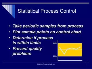
Example Recap: • The UCL and LCL have been calculated and were found to equal: • UCL = 0.86 • LCL = 0.18 • What does this mean? One would expect 99.73% of sample averages (n = 5) to lie within the range of the UCL and LCL due to normal variation. . . In other words, one could expect 99.73% of all sample averages to lie between 0.86 and 0.18
R Chart: • The next steps are to calculate the upper and lower control limits for the Range Chart • --The objective of the Range chart is to detect changes in variability • Recall: • UCL = (D4*R bar) • LCL = (D3*R bar)
Now complete the R Chart: • We have already found R bar to be = 0.59 • -so- • UCL = 2.114*0.59 • LCL = 0*0.59 • UCL = 1.25 • LCL = 0
SPC Monitoring Control Charts
Control Chart Interpretation Rules: • Look for Special Causes, which are suspect when: • 1.) One or more points are above the UCL or below the LCL • 2.) Seven or more consecutive points are above or below the centerline • 3.) One in twenty plotted points is in the 1/3 outer edge of the chart • 4.) Movements of five or more consecutive points are either up or down
Completed X bar R Charts: Special Cause
Special Cause Variation • If special causes are identified, the process is considered to be ‘unstable’ • Removing special causes when they are harmful (which is most of the time) is an important part of process improvement • Tracking down special causes often relies heavily on people’s (operators, supervisors, etc.) memories of what made that occurrence different
Special Cause Variation • When you spot a special cause: • Control any damage or problems with immediate (short term) fix • Once a ‘quick fix’ is in place, search for the cause • Once you determine the special cause, develop a longer-term remedy
Statistical Process Control Variables Data—The End