Statistical Process Control
Statistical Process Control. Lecture Outline. Basics of Statistical Process Control Control Charts Control Charts for Attributes Control Charts for Variables Control Chart Patterns SPC with Excel Process Capability. UCL. LCL. Basics of Statistical Process Control.

Statistical Process Control
E N D
Presentation Transcript
Lecture Outline • Basics of Statistical Process Control • Control Charts • Control Charts for Attributes • Control Charts for Variables • Control Chart Patterns • SPC with Excel • Process Capability
UCL LCL Basics of Statistical Process Control • Statistical Process Control (SPC) • monitoring production process to detect and prevent poor quality • Sample • subset of items produced to use for inspection • Control Charts • process is within statistical control limits
Random common causes inherent in a process can be eliminated only through improvements in the system Non-Random special causes due to identifiable factors can be modified through operator or management action Variability
SPC in TQM • SPC • tool for identifying problems and make improvements • contributes to the TQM goal of continuous improvements
Quality Measures • Attribute • a product characteristic that can be evaluated with a discrete response • good – bad; yes - no • Variable • a product characteristic that is continuous and can be measured • weight - length
Applying SPC to Service • Nature of defect is different in services • Service defect is a failure to meet customer requirements • Monitor times, customer satisfaction
Applying SPC to Service (cont.) • Hospitals • timeliness and quickness of care, staff responses to requests, accuracy of lab tests, cleanliness, courtesy, accuracy of paperwork, speed of admittance and checkouts • Grocery Stores • waiting time to check out, frequency of out-of-stock items, quality of food items, cleanliness, customer complaints, checkout register errors • Airlines • flight delays, lost luggage and luggage handling, waiting time at ticket counters and check-in, agent and flight attendant courtesy, accurate flight information, passenger cabin cleanliness and maintenance
Applying SPC to Service (cont.) • Fast-Food Restaurants • waiting time for service, customer complaints, cleanliness, food quality, order accuracy, employee courtesy • Catalogue-Order Companies • order accuracy, operator knowledge and courtesy, packaging, delivery time, phone order waiting time • Insurance Companies • billing accuracy, timeliness of claims processing, agent availability and response time
Where to Use Control Charts • Process has a tendency to go out of control • Process is particularly harmful and costly if it goes out of control • Examples • at the beginning of a process because it is a waste of time and money to begin production process with bad supplies • before a costly or irreversible point, after which product is difficult to rework or correct • before and after assembly or painting operations that might cover defects • before the outgoing final product or service is delivered
A graph that establishes control limits of a process Control limits upper and lower bands of a control chart Types of charts Attributes p-chart c-chart Variables range (R-chart) mean (x bar – chart) Control Charts
Out of control Upper control limit Process average Lower control limit 1 2 3 4 5 6 7 8 9 10 Sample number Process Control Chart
95% 99.74% -3 -2 -1 =0 1 2 3 Normal Distribution
A Process Is in Control If … … no sample points outside limits … most points near process average … about equal number of points above and below centerline … points appear randomly distributed
Control Charts for Attributes • p-charts • uses portion defective in a sample • c-charts • uses number of defects in an item
UCL = p + zp LCL = p - zp z = number of standard deviations from process average p = sample proportion defective; an estimate of process average p = standard deviation of sample proportion p(1 - p) n p = p-Chart
NUMBER OF PROPORTION SAMPLE DEFECTIVES DEFECTIVE 1 6 .06 2 0 .00 3 4 .04 : : : : : : 20 18 .18 200 20 samples of 100 pairs of jeans p-Chart Example
total defectives total sample observations p = = = p(1 - p) n UCL = p + z = UCL = p(1 - p) n LCL = p - z = LCL = p-Chart Example (cont.)
0.20 UCL = 0.190 0.18 0.16 0.14 0.12 p = 0.10 Proportion defective 0.10 0.08 0.06 0.04 0.02 LCL = 0.010 2 4 6 8 10 12 14 16 18 20 Sample number p-Chart Example (cont.)
UCL = c + zc c = c LCL = c - zc where c = number of defects per sample c-Chart
Number of defects in 15 sample rooms NUMBER OF DEFECTS SAMPLE c = = 1 12 2 8 3 16 : : : : 15 15 190 UCL = c + zc = = LCL = c + zc = = c-Chart (cont.)
24 UCL = 23.35 21 18 c = 12.67 15 Number of defects 12 9 6 LCL = 1.99 3 2 4 6 8 10 12 14 16 Sample number c-Chart (cont.)
Control Charts for Variables • Mean chart ( x -Chart ) • uses average of a sample • Range chart ( R-Chart ) • uses amount of dispersion in a sample
x1 + x2 + ... xk k = x = = = UCL = x + A2R LCL = x - A2R where x = average of sample means = x-bar Chart
OBSERVATIONS (SLIP- RING DIAMETER, CM) SAMPLE k1 2 3 4 5 x R 1 5.02 5.01 4.94 4.99 4.96 4.98 0.08 2 5.01 5.03 5.07 4.95 4.96 5.00 0.12 3 4.99 5.00 4.93 4.92 4.99 4.97 0.08 4 5.03 4.91 5.01 4.98 4.89 4.96 0.14 5 4.95 4.92 5.03 5.05 5.01 4.99 0.13 6 4.97 5.06 5.06 4.96 5.03 5.01 0.10 7 5.05 5.01 5.10 4.96 4.99 5.02 0.14 8 5.09 5.10 5.00 4.99 5.08 5.05 0.11 9 5.14 5.10 4.99 5.08 5.09 5.08 0.15 10 5.01 4.98 5.08 5.07 4.99 5.03 0.10 50.09 1.15 x-bar Chart Example Example 15.4
x k = x = = = cm UCL = x + A2R = = LCL = x - A2R = = = = x- bar Chart Example (cont.) Retrieve Factor Value A2
5.10 – 5.08 – 5.06 – 5.04 – 5.02 – 5.00 – 4.98 – 4.96 – 4.94 – 4.92 – UCL = 5.08 = x = 5.01 Mean LCL = 4.94 | 1 | 2 | 3 | 4 | 5 | 6 | 7 | 8 | 9 | 10 Sample number x- bar Chart Example (cont.)
UCL = D4R LCL = D3R • R k R = where R = range of each sample k = number of samples R- Chart
OBSERVATIONS (SLIP-RING DIAMETER, CM) SAMPLE k1 2 3 4 5 x R 1 5.02 5.01 4.94 4.99 4.96 4.98 0.08 2 5.01 5.03 5.07 4.95 4.96 5.00 0.12 3 4.99 5.00 4.93 4.92 4.99 4.97 0.08 4 5.03 4.91 5.01 4.98 4.89 4.96 0.14 5 4.95 4.92 5.03 5.05 5.01 4.99 0.13 6 4.97 5.06 5.06 4.96 5.03 5.01 0.10 7 5.05 5.01 5.10 4.96 4.99 5.02 0.14 8 5.09 5.10 5.00 4.99 5.08 5.05 0.11 9 5.14 5.10 4.99 5.08 5.09 5.08 0.15 10 5.01 4.98 5.08 5.07 4.99 5.03 0.10 50.09 1.15 R-Chart Example Example 15.3
R k UCL = D4R = = LCL = D3R = = R = = = R-Chart Example (cont.) Retrieve Factor Values D3 and D4 Example 15.3
0.28 – 0.24 – 0.20 – 0.16 – 0.12 – 0.08 – 0.04 – 0 – UCL = 0.243 R = 0.115 Range LCL = 0 | 1 | 2 | 3 | 4 | 5 | 6 | 8 | 9 | 10 | 7 Sample number R-Chart Example (cont.)
Using x- bar and R-Charts Together • Process average and process variability must be in control. • It is possible for samples to have very narrow ranges, but their averages is beyond control limits. • It is possible for sample averages to be in control, but ranges might be very large.
UCL UCL LCL LCL Sample observations consistently below the center line Sample observations consistently above the center line Control Chart Patterns
UCL UCL LCL Sample observations consistently increasing LCL Sample observations consistently decreasing Control Chart Patterns (cont.)
= UCL 3 sigma = x + A2R Zone A = 2 3 2 sigma = x + (A2R) Zone B = 1 3 1 sigma = x + (A2R) Zone C = Process average x Zone C = 1 3 1 sigma = x - (A2R) Zone B = 2 3 2 sigma = x - (A2R) Zone A = LCL 3 sigma = x - A2R | 1 | 2 | 3 | 4 | 5 | 6 | 7 | 8 | 9 | 10 | 11 | 12 | 13 Sample number Zones for Pattern Tests
Process Capability • Tolerances • design specifications reflecting product requirements • Process capability • range of natural variability in a process what we measure with control charts
Design Specifications (a) Natural variation exceeds design specifications; process is not capable of meeting specifications all the time. Process Design Specifications (b) Design specifications and natural variation the same; process is capable of meeting specifications most of the time. Process Process Capability
Design Specifications (c) Design specifications greater than natural variation; process is capable of always conforming to specifications. Process Design Specifications (d) Specifications greater than natural variation, but process off center; capable but some output will not meet upper specification. Process Process Capability (cont.)
Process Capability Ratio tolerance range process range Cp = = upper specification limit - lower specification limit 6 Process Capability Measures
Net weight specification = 9.0 oz 0.5 oz Process mean = 8.80 oz Process standard deviation = 0.12 oz upper specification limit - lower specification limit 6 Cp = = = Computing Cp
Process Capability Index = x - lower specification limit 3 , Cpk = minimum = upper specification limit - x 3 Process Capability Measures
= x - lower specification limit 3 , Cpk = minimum = minimum , = = upper specification limit - x 3 Computing Cpk Net weight specification = 9.0 oz 0.5 oz Process mean = 8.80 oz Process standard deviation = 0.12 oz