Statistical Process Control

Statistical Process Control S6 PowerPoint presentation to accompany Heizer and Render Operations Management, 10e Principles of Operations Management, 8e PowerPoint slides by Jeff Heyl © 2011 Pearson Education, Inc. publishing as Prentice Hall

Statistical Process Control The objective of a process control system is to provide a statistical signal when assignable causes of variation are present © 2011 Pearson Education, Inc. publishing as Prentice Hall

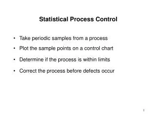
Statistical Process Control (SPC) • Variability is inherent in every process • Natural or common causes • Special or assignable causes • Provides a statistical signal when assignable causes are present • Detect and eliminate assignable causes of variation © 2011 Pearson Education, Inc. publishing as Prentice Hall

Natural Variations • Also called common causes • Affect virtually all production processes • Expected amount of variation • Output measures follow a probability distribution • For any distribution there is a measure of central tendency and dispersion • If the distribution of outputs falls within acceptable limits, the process is said to be “in control” © 2011 Pearson Education, Inc. publishing as Prentice Hall

Assignable Variations • Also called special causes of variation • Generally this is some change in the process • Variations that can be traced to a specific reason • The objective is to discover when assignable causes are present • Eliminate the bad causes • Incorporate the good causes © 2011 Pearson Education, Inc. publishing as Prentice Hall

Each of these represents one sample of five boxes of cereal # # # # # Frequency # # # # # # # # # # # # # # # # # # # # # Weight Samples To measure the process, we take samples and analyze the sample statistics following these steps (a) Samples of the product, say five boxes of cereal taken off the filling machine line, vary from each other in weight Figure S6.1 © 2011 Pearson Education, Inc. publishing as Prentice Hall

The solid line represents the distribution Frequency Weight Samples To measure the process, we take samples and analyze the sample statistics following these steps (b) After enough samples are taken from a stable process, they form a pattern called a distribution Figure S6.1 © 2011 Pearson Education, Inc. publishing as Prentice Hall

Central tendency Variation Shape Frequency Weight Weight Weight Samples To measure the process, we take samples and analyze the sample statistics following these steps (c) There are many types of distributions, including the normal (bell-shaped) distribution, but distributions do differ in terms of central tendency (mean), standard deviation or variance, and shape Figure S6.1 © 2011 Pearson Education, Inc. publishing as Prentice Hall

Frequency Prediction Time Weight Samples To measure the process, we take samples and analyze the sample statistics following these steps (d) If only natural causes of variation are present, the output of a process forms a distribution that is stable over time and is predictable Figure S6.1 © 2011 Pearson Education, Inc. publishing as Prentice Hall

? ? ? ? ? ? ? ? ? ? ? ? ? ? ? ? ? ? ? Prediction Frequency Time Weight Samples To measure the process, we take samples and analyze the sample statistics following these steps (e) If assignable causes are present, the process output is not stable over time and is not predicable Figure S6.1 © 2011 Pearson Education, Inc. publishing as Prentice Hall

Control Charts Constructed from historical data, the purpose of control charts is to help distinguish between natural variations and variations due to assignable causes © 2011 Pearson Education, Inc. publishing as Prentice Hall

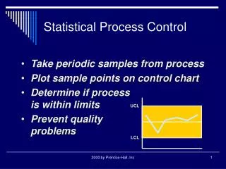
(a) In statistical control and capable of producing within control limits Frequency Upper control limit Lower control limit (b) In statistical control but not capable of producing within control limits (c) Out of control Size (weight, length, speed, etc.) Process Control Figure S6.2 © 2011 Pearson Education, Inc. publishing as Prentice Hall

Types of Data Variables Attributes • Characteristics that can take any real value • May be in whole or in fractional numbers • Continuous random variables • Defect-related characteristics • Classify products as either good or bad or count defects • Categorical or discrete random variables © 2011 Pearson Education, Inc. publishing as Prentice Hall

The mean of the sampling distribution (x) will be the same as the population mean m x = m The standard deviation of the sampling distribution (sx) will equal the population standard deviation (s) divided by the square root of the sample size, n s n sx = Central Limit Theorem Regardless of the distribution of the population, the distribution of sample means drawn from the population will tend to follow a normal curve © 2011 Pearson Education, Inc. publishing as Prentice Hall

Three population distributions Mean of sample means = x Beta Standard deviation of the sample means s n Normal = sx = Uniform | | | | | | | -3sx -2sx -1sxx +1sx +2sx +3sx 95.45% fall within ± 2sx 99.73% of all x fall within ± 3sx Population and Sampling Distributions Distribution of sample means Figure S6.3 © 2011 Pearson Education, Inc. publishing as Prentice Hall

For variables that have continuous dimensions • Weight, speed, length, strength, etc. • x-charts are to control the central tendency of the process • R-charts are to control the dispersion of the process • These two charts must be used together Control Charts for Variables © 2011 Pearson Education, Inc. publishing as Prentice Hall

For x-Charts when we know s Upper control limit (UCL) = x + zsx Lower control limit (LCL) = x - zsx where x = mean of the sample means or a target value set for the process z = number of normal standard deviations sx = standard deviation of the sample means = s/ n s = population standard deviation n = sample size Setting Chart Limits © 2011 Pearson Education, Inc. publishing as Prentice Hall

Hour 1 Sample Weight of Number Oat Flakes 1 17 2 13 3 16 4 18 5 17 6 16 7 15 8 17 9 16 Mean 16.1 s = 1 Hour Mean Hour Mean 1 16.1 7 15.2 2 16.8 8 16.4 3 15.5 9 16.3 4 16.5 10 14.8 5 16.5 11 14.2 6 16.4 12 17.3 n = 9 UCLx = x + zsx = 16 + 3(1/3) = 17 ozs LCLx = x - zsx = 16 - 3(1/3) = 15 ozs Setting Control Limits For 99.73% control limits, z = 3 © 2011 Pearson Education, Inc. publishing as Prentice Hall

Variation due to assignable causes Out of control 17 = UCL Variation due to natural causes 16 = Mean 15 = LCL Variation due to assignable causes | | | | | | | | | | | | 1 2 3 4 5 6 7 8 9 10 11 12 Out of control Sample number Setting Control Limits Control Chart for sample of 9 boxes © 2011 Pearson Education, Inc. publishing as Prentice Hall

For x-Charts when we don’t know s Upper control limit (UCL) = x + A2R Lower control limit (LCL) = x - A2R where R = average range of the samples A2 = control chart factor found in Table S6.1 x = mean of the sample means Setting Chart Limits © 2011 Pearson Education, Inc. publishing as Prentice Hall

Sample Size Mean Factor Upper Range Lower Range n A2 D4 D3 2 1.880 3.268 0 3 1.023 2.574 0 4 .729 2.282 0 5 .577 2.115 0 6 .483 2.004 0 7 .419 1.924 0.076 8 .373 1.864 0.136 9 .337 1.816 0.184 10 .308 1.777 0.223 12 .266 1.716 0.284 Control Chart Factors Table S6.1 © 2011 Pearson Education, Inc. publishing as Prentice Hall

Process average x = 12 ounces Average range R = .25 Sample size n = 5 UCLx = x + A2R = 12 + (.577)(.25) = 12 + .144 = 12.144 ounces From Table S6.1 Setting Control Limits © 2011 Pearson Education, Inc. publishing as Prentice Hall

Process average x = 12 ounces Average range R = .25 Sample size n = 5 UCLx = x + A2R = 12 + (.577)(.25) = 12 + .144 = 12.144 ounces UCL = 12.144 Mean = 12 LCLx = x - A2R = 12 - .144 = 11.857 ounces LCL = 11.857 Setting Control Limits © 2011 Pearson Education, Inc. publishing as Prentice Hall

UCL = 11.524 x – 10.959 LCL – 10.394 11.5 – 11.0 – 10.5 – x Bar Chart Sample Mean | | | | | | | | | 1 3 5 7 9 11 13 15 17 0.8 – 0.4 – 0.0 – Range Chart UCL = 0.6943 R = 0.2125 LCL = 0 Sample Range | | | | | | | | | 1 3 5 7 9 11 13 15 17 Restaurant Control Limits For salmon filets at Darden Restaurants © 2011 Pearson Education, Inc. publishing as Prentice Hall

Capability Histogram LSL USL Capability Mean = 10.959 Std.dev = 1.88 Cp = 1.77 Cpk = 1.7 10.2 10.5 10.8 11.1 11.4 11.7 12.0 Restaurant Control Limits Specifications LSL 10 USL 12 © 2011 Pearson Education, Inc. publishing as Prentice Hall

R – Chart • Type of variables control chart • Shows sample ranges over time • Difference between smallest and largest values in sample • Monitors process variability • Independent from process mean © 2011 Pearson Education, Inc. publishing as Prentice Hall

Upper control limit (UCLR) = D4R Lower control limit (LCLR) = D3R where R = average range of the samples D3 and D4 = control chart factors from Table S6.1 Setting Chart Limits For R-Charts © 2011 Pearson Education, Inc. publishing as Prentice Hall

Average range R = 5.3 pounds Sample size n = 5 From Table S6.1 D4 = 2.115, D3 = 0 UCLR = D4R = (2.115)(5.3) = 11.2 pounds UCL = 11.2 Mean = 5.3 LCLR = D3R = (0)(5.3) = 0 pounds LCL = 0 Setting Control Limits © 2011 Pearson Education, Inc. publishing as Prentice Hall

(a) These sampling distributions result in the charts below (Sampling mean is shifting upward but range is consistent) UCL (x-chart detects shift in central tendency) x-chart LCL UCL (R-chart does not detect change in mean) R-chart LCL Mean and Range Charts Figure S6.5 © 2011 Pearson Education, Inc. publishing as Prentice Hall

(b) These sampling distributions result in the charts below (Sampling mean is constant but dispersion is increasing) UCL (x-chart does not detect the increase in dispersion) x-chart LCL UCL (R-chart detects increase in dispersion) R-chart LCL Mean and Range Charts Figure S6.5 © 2011 Pearson Education, Inc. publishing as Prentice Hall

Steps In Creating Control Charts Take samples from the population and compute the appropriate sample statistic Use the sample statistic to calculate control limits and draw the control chart Plot sample results on the control chart and determine the state of the process (in or out of control) Investigate possible assignable causes and take any indicated actions Continue sampling from the process and reset the control limits when necessary © 2011 Pearson Education, Inc. publishing as Prentice Hall

Managerial Issues andControl Charts • Select points in the processes that need SPC • Determine the appropriate charting technique • Set clear policies and procedures Three major management decisions: © 2011 Pearson Education, Inc. publishing as Prentice Hall

Variables Data Using an x-Chart and R-Chart • Observations are variables • Collect 20 - 25 samples of n = 4, or n = 5, or more, each from a stable process and compute the mean for the x-chart and range for the R-chart • Track samples of n observations each. Which Control Chart to Use Table S6.3 © 2011 Pearson Education, Inc. publishing as Prentice Hall

Upper control limit Target Lower control limit Patterns in Control Charts One plot out above (or below). Investigate for cause. Process is “out of control.” Figure S6.7 © 2011 Pearson Education, Inc. publishing as Prentice Hall

Upper control limit Target Lower control limit Patterns in Control Charts Trends in either direction, 5 plots. Investigate for cause of progressive change. Figure S6.7 © 2011 Pearson Education, Inc. publishing as Prentice Hall

Upper control limit Target Lower control limit Patterns in Control Charts Two plots very near lower (or upper) control. Investigate for cause. Figure S6.7 © 2011 Pearson Education, Inc. publishing as Prentice Hall

Upper control limit Target Lower control limit Patterns in Control Charts Run of 5 above (or below) central line. Investigate for cause. Figure S6.7 © 2011 Pearson Education, Inc. publishing as Prentice Hall

Process Capability • The natural variation of a process should be small enough to produce products that meet the standards required • A process in statistical control does not necessarily meet the design specifications • Process capability is a measure of the relationship between the natural variation of the process and the design specifications © 2011 Pearson Education, Inc. publishing as Prentice Hall

Upper Specification - Lower Specification 6s Cp = Process Capability Ratio • A capable process must have a Cp of at least 1.0 • Does not look at how well the process is centered in the specification range • Often a target value of Cp = 1.33 is used to allow for off-center processes • Six Sigma quality requires a Cp = 2.0 © 2011 Pearson Education, Inc. publishing as Prentice Hall

Process mean x = 210.0 minutes Process standard deviation s = .516 minutes Design specification = 210 ± 3 minutes Upper Specification - Lower Specification 6s Cp = Process Capability Ratio Insurance claims process © 2011 Pearson Education, Inc. publishing as Prentice Hall

Process mean x = 210.0 minutes Process standard deviation s = .516 minutes Design specification = 210 ± 3 minutes Upper Specification - Lower Specification 6s Cp = 213 - 207 6(.516) = = 1.938 Process Capability Ratio Insurance claims process © 2011 Pearson Education, Inc. publishing as Prentice Hall

Process mean x = 210.0 minutes Process standard deviation s = .516 minutes Design specification = 210 ± 3 minutes Upper Specification - Lower Specification 6s Cp = 213 - 207 6(.516) = = 1.938 Process Capability Ratio Insurance claims process Process is capable © 2011 Pearson Education, Inc. publishing as Prentice Hall

UpperSpecification - xLimit 3s Lowerx - Specification Limit 3s Cpk = minimum of , Process Capability Index • A capable process must have a Cpk of at least 1.0 • A capable process is not necessarily in the center of the specification, but it falls within the specification limit at both extremes © 2011 Pearson Education, Inc. publishing as Prentice Hall

New process mean x = .250 inches Process standard deviation s = .0005 inches Upper Specification Limit = .251 inches Lower Specification Limit = .249 inches Process Capability Index New Cutting Machine © 2011 Pearson Education, Inc. publishing as Prentice Hall

New process mean x = .250 inches Process standard deviation s = .0005 inches Upper Specification Limit = .251 inches Lower Specification Limit = .249 inches (.251) - .250 (3).0005 Cpk = minimum of , Process Capability Index New Cutting Machine © 2011 Pearson Education, Inc. publishing as Prentice Hall

Statistical Process Control